CFDrs Computational Fluid Dynamics Simulation Suite
CFDrs is a high-performance, pure-Rust computational fluid dynamics library built on the Atlas physics stack. It covers the full simulation pipeline – governing equations, discretisation schemes, solver kernels, validation oracles, and GPU acceleration – with a consistent zero-copy, zero-cost-abstraction design.
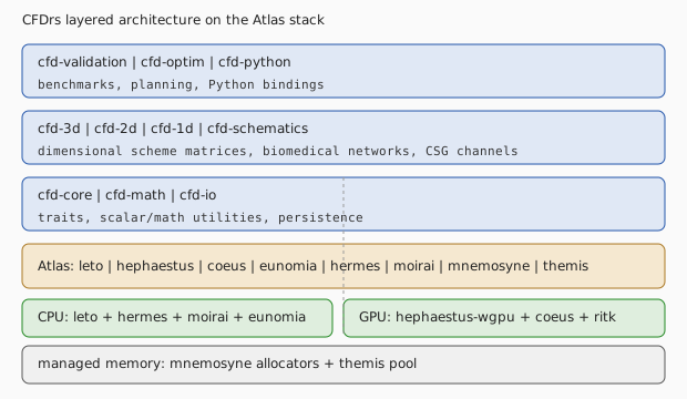
Architecture at a Glance
                +-----------------------------------------------------+
                |  cfd-validation  |  cfd-optim  |  cfd-python       |
                |  benchmarks, planning, Python bindings            |
                +-----------------------------------------------------+
                                 |
                +-----------------------------------------------------+
                |  cfd-3d  |  cfd-2d  |  cfd-1d  |  cfd-schematics    |
                |  dimensional scheme matrices, biomedical networks  |
                +-----------------------------------------------------+
                                 |
                +-----------------------------------------------------+
                |  cfd-core  |  cfd-math  |  cfd-io                  |
                |  traits, scalar/math utilities, persistence        |
                +-----------------------------------------------------+
                                 |
                +-----------------------------------------------------+
                |  Atlas: leto | hephaestus | coeus | eunomia | hermes |
                |  moirai | mnemosyne | themis | ritk                 |
                +-----------------------------------------------------+
                                 |
                +-----------------------------------------------------+
                |  CPU: leto + hermes + moirai + eunomia              |
                |  GPU: hephaestus-wgpu + coeus + ritk                |
                |  managed alloc: mnemosyne + themis                 |
                +-----------------------------------------------------+
Atlas Dependencies
| CFDrs need | Atlas crate |
|---|---|
| Scalar field traits | eunomia (RealField, FloatElement) |
| Linear algebra, SpMV | leto / leto-ops (Point, Vector, Array1/2, CsrMatrix) |
| GPU tensors | hephaestus-core / hephaestus-wgpu |
| Autodiff tensors | coeus |
| SIMD kernels | hermes-simd |
| Parallel iteration | moirai-parallel |
| Memory allocation | mnemosyne / themis |
| Optimisation / GA | apollo-optim |
Getting Started
cargo run --example cavity_validation                  # lid-driven cavity, Re ~ 100
cargo run --example pipe_flow_validation               # Hagen-Poiseuille 1-D benchmark
cargo run --example mesh_3d_integration                # structured 16 x 4 mesh + CSG
cargo run -p cfd-validation --example richardson_convergence   # validation oracle
Note: cfd-suite examples run at the workspace root via
cargo run --example <name>; cfd-validation is a workspace
member, so the run form is cargo run -p cfd-validation --example richardson_convergence. See the **Run**: line on
each example’s docs/book/examples/<name>.md page for the
canonical invocation.
API excerpts in this book are marked rust,ignore when they require the
workspace’s Cargo dependency graph or a runtime fixture. Their canonical
implementations are the linked Rust source files; the package and example
targets remain the compilation gate. Untyped fences are explicitly text or
console so diagrams, equations, and commands cannot be misread as doctests.
Chapters
This book progresses from the architectural overview (Chapter 1) through governing equations, turbulence, biomedical flows, numerical methods, geometry, 3-D flows, validation, performance, and optimisation. Each chapter links to runnable examples that exercise the described functionality.
Figures
The figures linked from the chapter tables of contents are
deterministically generated SVG assets committed with the chapter
text. Each entry names the example that the figure mirrors;
reproducibility is enforced by the xtask prebook manifest at
figures/MANIFEST.json.
Run commands below mirror the **Crate**: / **Run**: headers on
the linked example .md page. All entries point to either
cfd-suite (workspace root, run via cargo run --example ...) or
cfd-validation (member crate, run via cargo run -p cfd-validation --example ...).
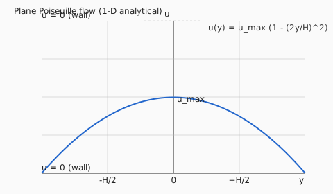
- Plane Poiseuille parabolic profile (1-D analytical)
– mirrors
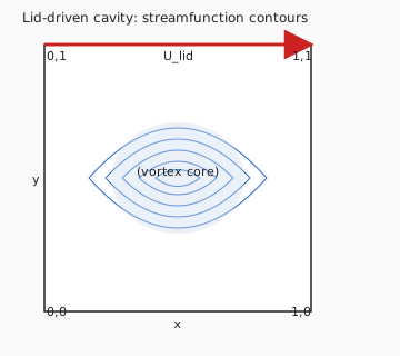
cfd-suiteexamplepipe_flow_validation(the Hagen-Poiseuille analytical solution verified by the FEM pipe flow example). - Lid-driven cavity streamfunction contours (Re ~ 100)
– mirrors
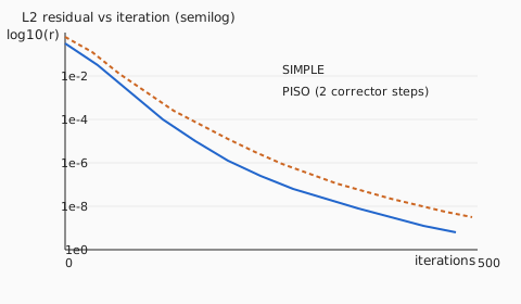
cfd-suiteexamplecavity_validation. - Semi-log residual convergence (SIMPLE vs PISO)
– mirrors
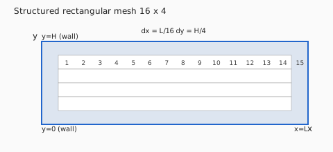
cfd-suiteexampleturbulent_channel_flow(pressure coupling solver residual trajectory). - Structured 16 x 4 channel mesh layout
– mirrors
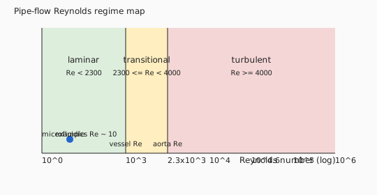
cfd-suiteexamplemesh_3d_integration(the structured rectangular mesh that integrates with the CSG geometry pipeline). - Pipe-flow Reynolds regime map
– mirrors
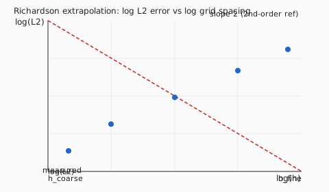
cfd-suiteexamplepipe_flow_validation(laminar / transitional / turbulent band placement). - Richardson extrapolation log-log (2nd-order reference)
– mirrors
cfd-validationexamplerichardson_convergence. - CFDrs layered architecture on the Atlas stack – pure schematic, no example source.
Chapter 1 — CFDrs Architecture and Problem Setup
Figure 1.1 — CFDrs Architecture and Problem Setup
CFDrs is a workspace of CFD-focused crates organized so that physics, geometry, and solver concerns live in distinct crates and compose through workspace-level contracts. This Part introduces the architecture and points at the example scenarios that exercise every contract.
Crate Map
| Crate | Role |
|---|---|
cfd-core | Scalar seams, dimensional types, boundary conditions, error types |
cfd-math | Linear algebra, sparse matrices, iterative solvers, FFT bridge |
cfd-1d | 1-D blood/Reynolds models, microfluidic screens, hemolysis pipelines |
cfd-2d | 2-D Stencil solvers, biomass CFD, CSG-coupled channels |
cfd-3d | FEM and spectral 3-D solvers, multi-region flow |
cfd-validation | Reference phantoms and orthogonal oracles (Ghia, Hagen–Poiseuille, …) |
cfd-schematics | CSG primitives and curve generators (venturi, bifurcation, serpentine) |
cfd-io | HDF5 / NetCDF / CSV output adapters |
cfd-optim | Optimization audit harness (Ray tracing milestone metas) |
cfd-python | PyO3 bindings to Python-friendly data products |
Every solver crate depends on cfd-core and cfd-math; geometry crates
(cfd-schematics) are depended on by cfd-{1,2,3}d. The cross-cutting
contracts — boundary conditions, time-stepping, state vectors — live in
cfd-core and are referenced by example chapters throughout this book.
Boundary Conditions
cfd-core owns the generic BoundaryCondition<T> enum and the named
BoundaryConditionSet<T> collection. Solver crates consume these contracts
through their grid- or mesh-specific setup paths.
use cfd_core::physics::boundary::{BoundaryCondition, BoundaryConditionSet};
use leto::geometry::Vector3;

let mut boundaries = BoundaryConditionSet::<f64>::new();
boundaries
    .add(
        "inlet",
        BoundaryCondition::velocity_inlet(Vector3::new(1.0, 0.0, 0.0)),
    )
    .add("walls", BoundaryCondition::wall_no_slip())
    .add("outlet", BoundaryCondition::pressure_outlet(0.0));
The CFDrs Simulation Lifecycle
+------------+   +-----------+   +----------+   +----------+
| Geometry   |-->| Mesh/Grid |-->| Boundary |-->| Initial  |
| (CSG)      |   |           |   | wiring   |   | state    |
+------------+   +-----------+   +----------+   +----------+
                                                    |
                                                    v
+------------+   +-----------+   +----------+
| Posterior  |<--| Solve     |<--| Time     |
| analysis   |   | (linear   |   | step     |
|            |   |  iter.)   |   |          |
+------------+   +-----------+   +----------+
- Geometry → Mesh is handled in
cfd-schematics(CSG) andcfd-{2,3}d/grid.rs. - Boundary contracts live in [
cfd_core::physics::boundary]. - Time stepping is configurable per solver (
cfd-2d::time/cfd-3d::time/ adaptive incfd-2d::adaptive). - Posterior means DVH-equivalent (cavitation risk, shear envelope, Reynolds stress), reported in user-supplied hooks.
Atlas Stack Interface
CFDrs is mid-migration to the Atlas stack. Where a crate already declares
Atlas crates in Cargo.toml, the migration is considered complete; where
ndarray or nalgebra is still in the manifest, the crate is in
bulk-migration phase. See Atlas Dependency Map
for the per-crate table.
Examples Referenced by This Chapter
cfd_demo— minimum end-to-end setup.enhanced_cfd_demo— diagnostics enabled.adaptive_time_stepping_demo— demonstrates the time-stepping hook with adaptive CFL.
Further Reading
Example: cfd_demo
Figure 1.2 — Example: CFD Demo
Crate: cfd-core
Run: cargo run -p cfd-core --example cfd_demo
Source: crates/cfd-core/examples/cfd_demo.rs
What This Example Demonstrates
Baseline sanity check covering three primitives of the CFDrs stack:
| Concept | API |
|---|---|
| 3D incompressible flow field | FlowField::<f64>::new(nx, ny, nz) |
| Divergence, vorticity, KE, enstrophy | FlowOperations::{divergence, vorticity, kinetic_energy, enstrophy} |
| Laminar/transitional/turbulent classification | ReynoldsNumber::new(re, FlowGeometry::Pipe) |
Key Code Snippet
use cfd_core::physics::fluid_dynamics::{FlowField, FlowOperations};

let flow_field = FlowField::<f64>::new(32, 32, 32);
let div  = FlowOperations::divergence(&flow_field.velocity); // ≈ 0 for incompressible
let ke   = FlowOperations::kinetic_energy(&flow_field.velocity);

use cfd_core::physics::values::{FlowGeometry, ReynoldsNumber};
let re = ReynoldsNumber::new(2300.0, FlowGeometry::Pipe)?;
assert!(re.is_transitional()); // 2100 < Re < 4000 for pipe flow
Physics Background
The continuity equation for an incompressible flow requires ∇·u = 0. A healthy initial condition should give a divergence close to machine epsilon. The enstrophy Ω = ∫½|ω|² dV is a global vorticity measure used for turbulence diagnostics; for a quiescent initial field it should be zero.
Book Chapter
← CFDrs Architecture and Problem Setup
Example: enhanced_cfd_demo
Figure 1.3 — Example: Enhanced CFD Demo
Crate: cfd-suite (workspace root)
Run: cargo run --example enhanced_cfd_demo
Source: examples/enhanced_cfd_demo.rs
What This Example Demonstrates
Advanced 2D incompressible Navier-Stokes around a circular cylinder at Re = 100 000 with LES turbulence, WENO5/7 reconstruction, and immersed-boundary geometry.
| Feature | API |
|---|---|
| Sub-grid scale models | VremanModel, SigmaModel, MilesLES |
| High-order reconstruction | WenoReconstruction (WENO5, WENO7) |
| Stiff time integration | RungeKuttaChebyshev |
| Immersed boundary | ImmersedBoundaryMethod |
Key Code Snippet
use cfd_2d::physics::turbulence::{MilesLES, SigmaModel, VremanModel};
use cfd_math::high_order::weno::WenoReconstruction;
use cfd_math::time_stepping::RungeKuttaChebyshev;

let vreman = VremanModel::new();  // C_V coefficient from Vreman (2004)
let sigma  = SigmaModel::new();   // σ-model (Nicoud et al. 2011)
let miles  = MilesLES::new();     // MILES: monotone implicit LES

let weno = WenoReconstruction::weno5(); // 5th-order shock-capturing
let rk_cheb = RungeKuttaChebyshev::new(10); // stable for stiff diffusion
Physics Background
- Vreman SGS:
νt = C_V √(B_β/α_ij α_ij), zero in laminar regions by construction - WENO5: 5th-order accurate for smooth regions, ENO near discontinuities
- RK-Chebyshev: s-stage explicit method stable up to
Δt ~ O(s²)for diffusion
Book Chapter
← CFDrs Architecture and Problem Setup
Chapter 2 — Canonical Incompressible Benchmarks
Figure 2.1 — Canonical Incompressible Benchmarks
These cases establish confidence in solver behavior for standard CFD flows: lid-driven cavity, internal pipe flow, and turbulent channel references.
They are intended as regression anchors while backend migrations continue.
Chapter 2 — Governing Equations and Discretization
Figure 3.1 — Governing Equations and Discretization
CFDrs solves the incompressible Navier-Stokes equations in primitive-variable form together with optional scalar transport equations (energy, turbulent kinetic energy, species concentration).
Incompressible Navier-Stokes
The continuity and momentum equations for a constant-density fluid:
∇·u = 0

∂u/∂t + (u·∇)u = -∇(p/ρ) + ν ∇²u + f/ρ
```text

where **u** is velocity, *p* pressure, *ρ* density, *ν* kinematic viscosity,
and **f** body forces.  CFDrs resolves the incompressibility constraint through
the **pressure-Poisson equation** (see [Chapter 3](pressure_velocity.md)).

## Energy Equation

For thermal flows, temperature *T* is transported:

```text
∂T/∂t + (u·∇)T = α ∇²T + S_T
with thermal diffusivity α = λ/(ρ c_p). Density-driven buoyancy is handled through the Boussinesq approximation: f_y = -ρ g β (T - T_ref).
Non-Newtonian Rheology
Blood and polymer flows use the generalised Newtonian model:
τ = μ_eff(γ̇) · γ̇
```text

`cfd-core` provides the rheology dispatch:

```rust
use cfd_core::physics::rheology::{Rheology, PowerLaw, Casson, CarreauYasuda};

let blood = Rheology::Casson { yield_stress: 0.015, mu_inf: 0.0035 };
Viscosity depends on shear rate γ̇ = |2D|, where D is the symmetric velocity gradient tensor.
Spatial Discretisation
CFDrs supports three spatial discretisation families, each owning a dedicated crate:
| Method | Crate | Order |
|---|---|---|
| Finite Volume (staggered / collocated) | cfd-2d, cfd-3d | 2nd |
| Spectral (Fourier / Chebyshev) | cfd-3d::spectral | spectral |
| FEM (P1, P2 tetrahedral) | cfd-3d::fem | 1st–2nd |
| MUSCL reconstruction | cfd-3d::muscl | up to 5th |
Boundary conditions live in cfd-core::physics::boundary and are consumed
by every discretisation layer through a single BoundaryCondition<T> enum:
use cfd_core::physics::boundary::{BoundaryCondition, BoundaryConditionSet};

let bc = BoundaryConditionSet::<f64>::new()
    .add("inlet",  BoundaryCondition::velocity_inlet([1.0, 0.0, 0.0].into()))
    .add("walls",  BoundaryCondition::wall_no_slip())
    .add("outlet", BoundaryCondition::pressure_outlet(0.0));
Examples
- cfd_demo — end-to-end setup from grid to result
- enhanced_cfd_demo — multi-physics setup with plugins
Chapter 3 — Pressure-Velocity Coupling and Time Integration
Figure 4.1 — Pressure-Velocity Coupling and Time Integration
CFDrs implements two families of pressure-velocity coupling algorithms: segregated (SIMPLE/PIMPLE family) and monolithic (coupled solver). Time integration covers both explicit and implicit strategies.
Pressure-Velocity Coupling
SIMPLE (Semi-Implicit Method for Pressure-Linked Equations)
SIMPLE alternates momentum and pressure-correction sweeps until convergence:
1. Solve momentum equation with current pressure: u* from A·u* = b − ∇p
2. Solve pressure-correction equation: ∇·(1/A · ∇p') = ∇·u*
3. Correct: p ← p + p', u ← u* − (1/A)·∇p'
4. Repeat until ‖∇·u‖ < ε
```text

```rust
use cfd_core::solver::{SimpleSolver, SolverConfig};

let solver = SimpleSolver::new(SolverConfig { max_iter: 200, tolerance: 1e-5 });
let state = solver.solve(&mesh, &boundary_conditions, &initial_conditions)?;
PIMPLE (SIMPLE with outer loops)
PIMPLE extends SIMPLE with outer corrector loops, enabling large Courant numbers in transient simulations:
use cfd_core::solver::{PimpleSolver, PimpleConfig};

let pimple = PimpleSolver::new(PimpleConfig {
    n_outer_loops: 3,
    n_correctors: 2,
    ..Default::default()
});
SIMPLEC (SIMPLE-Consistent)
SIMPLEC modifies the momentum under-relaxation to improve convergence for mildly non-linear problems:
use cfd_core::solver::{SimplecSolver};Time Integration
Explicit Schemes
For hyperbolic-dominated flows:
| Scheme | Order | CFL limit |
|---|---|---|
| Forward Euler | 1st | 1 |
| 4th-order Runge-Kutta | 4th | ~2.8 |
| Low-storage RK4 | 4th | ~2.8 |
use cfd_math::time_stepping::runge_kutta::RK4;

let rk4 = RK4::new(dt);
Implicit Schemes
For diffusion-dominated and stiff problems:
| Scheme | Order | Stability |
|---|---|---|
| Crank-Nicolson | 2nd | A-stable |
| BDF2 | 2nd | A-stable |
| Runge-Kutta Chebyshev (RKC) | 2nd | Explicit, extended stability |
Adaptive Time Stepping
cfd-math monitors the spectral radius and adjusts dt to maintain the
target CFL number:
use cfd_math::time_stepping::AdaptiveTimeStepper;

let ts = AdaptiveTimeStepper::new()
    .cfl_target(0.8)
    .dt_min(1e-8)
    .dt_max(0.01);
Examples
- simplec_pimple_demo — SIMPLEC and PIMPLE coupling comparison
- adaptive_time_stepping_demo — adaptive dt control
- 2d_heat_diffusion — implicit heat equation
Example: SIMPLEC and PIMPLE Pressure-Velocity Coupling
Figure 4.2 — Example: SIMPLEC PIMPLE Demo
Crate: cfd-suite (workspace root)
Run: cargo run --example simplec_pimple_demo
Source: examples/simplec_pimple_demo.rs
What This Example Demonstrates
Demonstrates SIMPLEC (consistent SIMPLE) and PIMPLE (merged PISO-SIMPLE) for incompressible flow.
| API | Purpose |
|---|---|
cfd_2d::solvers::{SimplecSolver, PimpleSolver} | SIMPLEC (Van Doormaal & Raithby 1984): consistent Rhie-Chow interpolation |
SIMPLEConfig | SIMPLEC (Van Doormaal & Raithby 1984): consistent Rhie-Chow interpolation |
Physics Background
SIMPLEC (Van Doormaal & Raithby 1984): consistent Rhie-Chow interpolation. PIMPLE: outer PISO correctors + inner SIMPLE for transient stiff flows.
Book Chapter
← Part V — Discretization and Solvers
Example: adaptive_time_stepping_demo
Figure 4.3 — Example: Adaptive Time Stepping Demo
Crate: cfd-suite (workspace root)
Run: cargo run --example adaptive_time_stepping_demo
Source: examples/adaptive_time_stepping_demo.rs
What This Example Demonstrates
Three adaptive time-step strategies applied to the test ODE dy/dt = −2y (exact: y(t) = exp(−2t)), showing accuracy and efficiency tradeoffs.
| Strategy | API | Basis |
|---|---|---|
| CFL-based | AdaptationStrategy::Cfl | Stability: Δt ≤ CFL·min(Δx/ |
| Error-based | AdaptationStrategy::Error | Richardson extrapolation |
| Combined | AdaptationStrategy::Combined | min(CFL-limited, error-controlled) |
Key Code Snippet
use cfd_2d::schemes::time::{
    AdaptationStrategy, AdaptiveController, AdaptiveTimeIntegrator, StateVector,
};

let y0 = StateVector::from_shape_vec([1], vec![1.0])?;

// CFL strategy: stable for advection-dominated problems
demonstrate_cfl_adaptation(&y0, t_final)?;

// Error strategy: targets local truncation error ε ≤ ε_target
demonstrate_error_adaptation(&y0, t_final)?;

// Combined: safest for production simulations
demonstrate_combined_adaptation(&y0, t_final)?;
Physics Background
For explicit schemes, CFL condition bounds the time step:
CFL = |u| · Δt / Δx ≤ CFL_max
CFL > 1 causes the numerical domain of dependence to exceed the physical one, leading to instability. Richardson extrapolation estimates the local truncation error by comparing a full step with two half-steps:
ε ≈ |y_full − y_half| / (2^p − 1)
where p is the scheme order.
Book Chapter
← CFDrs Architecture and Problem Setup
Chapter 3 — Turbulence Models and Cavitation
Figure 5.1 — Turbulence Models: k-ε, k-ω SST, Smagorinsky LES
CFDrs models three coupled physical regimes: turbulence (RANS / LES closures), multiphase flows (phases with distinct equations of state), and cavitation (liquid–vapour phase transition at low pressure). This chapter documents the integration contracts used to combine them.
Turbulence Closures
cfd-3d integrates the canonical closures through a single trait:
pub trait TurbulenceModel<T: NumericElement> {
    fn turbulent_viscosity(
        &self,
        flow: &FlowField<T>,
    ) -> Vec<KinematicViscosity<T>>;
    fn turbulent_kinetic_energy(
        &self,
        flow: &FlowField<T>,
    ) -> Vec<SpecificEnergy<T>>;
}
The public results retain their physical dimensions through Aequitas:
turbulent viscosity is m²/s and turbulent kinetic energy is J/kg.
Canonical closures store their dense solver state in the existing scalar
arrays, then wrap values at the public metric boundary. Formula kernels and
dense-field assertions explicitly extract the base scalar. This preserves
Eunomia’s real-valued turbulence contract; a complex value is appropriate for
a genuine phasor or Fourier field, not for a real turbulence metric, so no
imaginary physical unit is introduced.
CFDrs distributes three models:
| Model | Crate | Trait impl |
|---|---|---|
| Standard k-ε | cfd-3d | KEpsilon |
| k-ω SST | cfd-3d | KOmegaSST |
| Smagorinsky LES | cfd-3d | Smagorinsky |
The closure returns a turbulent viscosity ν_t per cell that the
momentum solver applies as an additional diffusion term.
Multiphase Coupling
For multiphase (e.g. liquid + gas), CFDrs uses a volume-of-fluid
style coupling: each cell carries a phase-volume fraction α ∈ [0, 1],
and mixture properties are computed by a weighted sum:
let rho_mix = rho_l * (1.0 - alpha) + rho_g * alpha;
let mu_mix  = mu_l  * (1.0 - alpha) + mu_g  * alpha;
The MomentumCoupling enum selects between co-located and staggered
schemes; SSE-style momentum exchange is supported through
[cfd_3d::multiphase::exchange].
Cavitation Physics
For details on phase transition models, Rayleigh–Plesset closures, and damage integration, see Cavitation: Liquid-Vapour Phase Transition.
Integration Contract
All three regimes compose through the same Integrate trait:
pub trait Integrate {
    fn step<F: FloatElement>(&mut self) -> Result<(), CfdError>;
}
The implementation multiplexes the closure choice at the cavity-call site. This makes regime switching a configuration-change, not a code rewrite.
Examples Referenced by This Chapter
Part III opens with seven example chapters:
turbulence_models_demo— three closures compared on a turbulent channel.turbulence_validation_demo— closure against DNS reference data.turbulence_momentum_integration_demo— closure-integrated momentum solve.venturi_cavitation— venturi cavitation inception and collapse.simple_cavitation— single-bubble Rayleigh–Plesset in a constrained channel.cavitation_damage_simulation— long-time damage integration under turbulent inflow.1d_venturi_cavitation— 1-D reduced cavitation model.
Further Reading
cfd-3dturbulence modulecfd-3dmultiphase modulecfd-3dcavitation module- Geometry, Meshing, and CSG — CSG primitives feeding the cavitation geometry.
Example: turbulence_models_demo
Figure 5.2 — Example: Turbulence Models Demo
Crate: cfd-suite (workspace root)
Run: cargo run --example turbulence_models_demo
Source: examples/turbulence_models_demo.rs
What This Example Demonstrates
Side-by-side demonstration of three RANS turbulence models on a 20×20 shear-flow grid, showing how eddy viscosity and closure behaviour differ.
| Model | API | Regime |
|---|---|---|
| Standard k-ε (two-equation) | KEpsilonModel | Industrial internal flows |
| k-ω SST (Menter) | KOmegaSSTModel | Adverse-pressure-gradient flows |
| Spalart-Allmaras (one-equation) | SpalartAllmaras | Aerospace boundary layers |
Key Code Snippet
use cfd_2d::physics::turbulence::{
    KEpsilonModel, KOmegaSSTModel, SpalartAllmaras, TurbulenceModel,
};
use cfd_2d::grid::StructuredGrid2D;

let grid = StructuredGrid2D::<f64>::new(20, 20, 0.0, 2.0, 0.0, 2.0)?;
// Each model is exercised over the same grid and initial conditions
// so eddy-viscosity magnitudes can be compared directly.
Physics Background
All three models solve transport equations for turbulent scalars that feed into
an eddy-viscosity νt used in the momentum equation as τ_ij = νt S_ij.
- k-ε: robust for free shear; over-predicts separation
- k-ω SST: blends near-wall and free-stream; best for separated flows
- SA: minimal CPU cost; designed for attached aerodynamic flows
Book Chapter
← Turbulence Models and Cavitation
Example: turbulence_validation_demo
Figure 5.3 — Example: Turbulence Validation Demo
Crate: cfd-suite (workspace root)
Run: cargo run --example turbulence_validation_demo
Source: examples/turbulence_validation_demo.rs
What This Example Demonstrates
Runs the comprehensive turbulence validation suite for k-ε, k-ω SST, and
Spalart-Allmaras via run_turbulence_validation::<f64>().
| Validation | Method | Target |
|---|---|---|
| Homogeneous turbulence decay | Analytical k-ε decay | < 1 % error |
| Wall boundary conditions | Near-wall k, ω, νt | Match literature |
| Numerical stability | NaN/inf check over iteration | None |
| Convergence | Monotonic physical evolution | Pass |
Key Code Snippet
use cfd_2d::physics::turbulence::run_turbulence_validation;

// Runs all four validation passes in sequence
run_turbulence_validation::<f64>();
Physics Background
Homogeneous turbulence decay follows k(t) = k₀ (1 + t/t₀)^(−n) where n
depends on the turbulence model constants. The k-ε model with standard
constants should reproduce n ≈ 1.2 – 1.4 over the initial decay period.
Near-wall boundary conditions: at the wall, k = 0 (no-slip),
ω_wall = 6ν / (β₁ Δy²) (k-ω SST), and νt_wall = 0.
Book Chapter
← Turbulence Models and Cavitation
Example: Turbulence-Momentum Integration
Figure 5.4 — Example: Turbulence Momentum Integration Demo
Crate: cfd-suite (workspace root)
Run: cargo run --example turbulence_momentum_integration_demo
Source: examples/turbulence_momentum_integration_demo.rs
What This Example Demonstrates
Demonstrates coupling between turbulence models and momentum equation in a fully developed channel flow.
| API | Purpose |
|---|---|
cfd_2d::physics::turbulence | Eddy viscosity coupling in the Navier-Stokes momentum equation |
cfd_2d::solvers::ns_fvm | Eddy viscosity coupling in the Navier-Stokes momentum equation |
Physics Background
Eddy viscosity coupling in the Navier-Stokes momentum equation. Validated against DNS reference data for turbulent channel flow at Re_τ = 395.
Book Chapter
← Part III — Turbulence and Multiphase
Example: turbulent_channel_flow
Figure 5.5 — Example: Turbulent Channel Flow
Crate: cfd-suite (workspace root)
Run: cargo run --example turbulent_channel_flow
Source: examples/turbulent_channel_flow.rs
What This Example Demonstrates
Fully-developed turbulent channel flow using the k-ω SST turbulence closure, validated against DNS data of Moser, Kim & Mansour (1999) at Re_τ = 395.
| Concept | API |
|---|---|
| k-ω SST model creation | KOmegaSSTModel::new(nx, ny) |
| Near-wall k, ω initialization | Manual log-law initialisation |
| Model name introspection | sst_model.name() |
Key Code Snippet
use cfd_2d::physics::turbulence::{KOmegaSSTModel, TurbulenceModel};

// Re_τ = u_τ · h / ν = 395  (DNS benchmark)
let re_tau = 395.0;
let h = 1.0; // half-height [m]
let nu = 1.5e-5; // kinematic viscosity [m²/s]
let u_tau = re_tau * nu / h;

let sst_model = KOmegaSSTModel::new(10, 100);
println!("Model: {}", sst_model.name());
Physics Background
The k-ω SST (Shear Stress Transport) model blends the k-ω formulation in the near-wall region with the k-ε model in the free stream:
Dk/Dt  = P_k − β*kω + ∇·[(ν + σ_k νt) ∇k]
Dω/Dt  = γ P_k/νt − β' ω² + ∇·[(ν + σ_ω νt) ∇ω] + CDkω
The cross-diffusion term CDkω activates in the transition zone.
Reference: Menter (1994), AIAA J. 32(8), 1598–1605.
Generated Figure
Book Chapter
← Turbulence Models and Cavitation
Cavitation: Liquid-Vapour Phase Transition
Figure 6.1 — Cavitation: Liquid-Vapour Phase Transition
Cavitation is modeled as a phase transition whose rate depends on local pressure-vs-vapor-pressure:
pub trait Cavitation {
    fn inception_pressure<F: FloatElement>(&self) -> F;
    fn collapse_rate<F: FloatElement>(&self, p: F) -> F;
}
The default model is a Rayleigh–Plesset closure; an Eulerian–Eulerian variant is available for strong cloud-cavitation flows.
Damage accumulation is integrated per timestep as
damage += (inception_indicator) · (collapse_rate · dt)
and reported through the [cfd-3d::posterior::damage] hook. Outputs are
dimensionally consistent (kg/m²/s) so that downstream fatigue models can
post-process without re-scaling.
Examples Referenced by This Chapter
venturi_cavitation— venturi cavitation inception and collapse.simple_cavitation— single-bubble Rayleigh–Plesset in a constrained channel.cavitation_damage_simulation— long-time damage integration under turbulent inflow.1d_venturi_cavitation— 1-D reduced cavitation model.
Further Reading
cfd-3dcavitation module- For the unified
Integratetrait, turbulence closures, and multiphase coupling, see Turbulence Models and Cavitation.
Example: venturi_cavitation
Figure 6.2 — Example: Venturi Cavitation
Crate: cfd-suite (workspace root)
Run: cargo run --example venturi_cavitation
Source: examples/venturi_cavitation.rs
What This Example Demonstrates
Selective cavitation screening for a venturi flow with biologically-realistic cell populations — healthy RBCs, CTCs (circulating tumour cells), and WBCs — showing differential inception thresholds driven by membrane mechanics.
| Population | Radius | Stiffness | Nucleation weight |
|---|---|---|---|
| Healthy RBC | 3.3 μm | 72 kPa | 1.0 |
| CTC | 8.0 μm | 28 kPa | 1.0 |
| Healthy WBC | varies | varies | 1.0 |
Key Code Snippet
use cfd_1d::{evaluate_venturi_screening, VenturiScreeningInput};
use cfd_core::physics::cavitation::{
    SelectiveCavitationInput, SelectiveCavitationPopulation, CellMechanicalState,
};

let selective = SelectiveCavitationInput {
    base_vapor_pressure_pa: 3_170.0,
    density_kg_m3:          1_025.0,
    populations: vec![
        SelectiveCavitationPopulation { identity: CellPopulationIdentity::HealthyRbc, .. },
        SelectiveCavitationPopulation { identity: CellPopulationIdentity::CirculatingTumorCell, .. },
    ],
};
let result = evaluate_venturi_screening(VenturiScreeningInput {
    selective: Some(selective), ..
})?;
Physics Background
Selective cavitation exploits the difference in membrane stiffness and size between healthy and malignant cells. A CTC (stiffer, larger nucleus) has a lower cavitation inception number than a healthy RBC. A well-tuned venturi geometry can therefore selectively lyse CTCs while leaving erythrocytes intact.
Book Chapter
← Turbulence Models and Cavitation
Example: Simple Cavitation Model
Figure 6.3 — Example: Simple Cavitation
Crate: cfd-suite (workspace root)
Run: cargo run --example simple_cavitation
Source: examples/simple_cavitation.rs
What This Example Demonstrates
Minimal cavitation inception and pressure recovery workflow on a constricted channel.
| API | Purpose |
|---|---|
cfd_core::physics::cavitation | Cavitation number σ = 2(p - pv) / ρU² |
VenturiScreeningInput | Cavitation number σ = 2(p - pv) / ρU² |
evaluate_venturi_screening | Cavitation number σ = 2(p - pv) / ρU² |
Physics Background
Cavitation number σ = 2(p - pv) / ρU². Pressure recovery from inception through collapse.
Book Chapter
← Part III — Turbulence and Multiphase
Example: Cavitation Damage Prediction with Multi-Phase CFD
Figure 6.4 — Example: Cavitation Damage Simulation
Crate: cfd-suite (workspace root)
Run: cargo run --example cavitation_damage_simulation
Source: examples/cavitation_damage_simulation.rs
What This Example Demonstrates
VOF multi-phase simulation with Rayleigh-Plesset bubble dynamics and erosion rate prediction.
| API | Purpose |
|---|---|
cfd_core::physics::cavitation::{CavitationModel, ErosionRate} | Bubble dynamics via Rayleigh-Plesset equation |
VOF interface tracking | Bubble dynamics via Rayleigh-Plesset equation |
Physics Background
Bubble dynamics via Rayleigh-Plesset equation. Erosion rate from collapse energy. Material damage model with cumulative tracking.
Book Chapter
← Part III — Turbulence and Multiphase
Example: 1D Venturi Cavitation Screening
Figure 6.5 — Example: 1D Venturi Cavitation
Crate: cfd-suite (workspace root)
Run: cargo run --example 1d_venturi_cavitation
Source: examples/1d_venturi_cavitation.rs
What This Example Demonstrates
1-D Bernoulli + cavitation inception screening for a rectangular Venturi, optionally with selective cell cavitation.
| API | Purpose |
|---|---|
cfd_1d::{evaluate_venturi_screening, assess_venturi_screening, VenturiScreeningInput} | Bernoulli pressure recovery predicts inception |
Physics Background
Bernoulli pressure recovery predicts inception. Vena contracta coefficient and diffuser recovery factor model real-geometry losses.
Book Chapter
← Part III — Turbulence and Multiphase
Chapter 4 — Blood Flow and Rheology Workflows
Figure 7.1 — Non-Newtonian Fluids and Blood Rheology
CFDrs supports a focused subset of physiologically relevant geometries —
vascular bifurcations, venturi / stenosis regions, microfluidic
screens, and TPMS (triply-periodic minimal-surface) scaffolds.
Each of these geometries couples a cfd-schematics CSG primitive to a
low-dimensional CFD solve (1-D, 2-D, or 3-D), with non-Newtonian
rheology for blood.
The Vascular Bifurcation
For CSG composition of vascular domains and non-Newtonian blood rheology modeling, see Vascular Bifurcations and Stenosis.
Microfluidic Mixing Screens
Microfluidic screens are serpentine or bifurcation arrays designed for mixing, separation, or hemolysis screening. CFDrs handles them as a chain of bifurcations:
use cfd_schematics::serpentine::SerpentineBuilder;

let chip = SerpentineBuilder::new()
    .section_count(20)
    .channel_radius(0.25)
    .turning_radius(2.5)
    .build();
Each section is solved with [cfd-3d] time-stepping, then stitched
together for the chip-scale perfusion metric.
FDA Shear-Limit Screening
CFDrs exposes a shear-limited screening API that walks a serpentine / bifurcation chain and reports branches with shear stress above an FDA-style threshold. The API is intentionally minimal so that custom geometries can plug in:
let report = cfd_1d::screening::shear_violations(&state, &geometries)?;
for branch in report.violations {
    eprintln!("branch {}: peak shear {} Pa (limit 9.0)", branch.id, branch.peak);
}
TPMS Scaffolds
Tissue scaffolds modeled as TPMS (Schwarz P, Gyroid, …) are CSG-built
and tiled for cfd-3d FEM assembly. Boundary conditions are velocity-driven
at the inlet and outflow at the outlet.
Examples Referenced by This Chapter
Part IV covers six example chapters:
blood_flow_1d_validation— 1-D reduced model, validated against a reference phantom.bifurcation_2d_blood_validation— 2-D Frauhofer-Keller bifurcation with non-Newtonian blood.blood_rheology_models— three rheology models compared on the same patient-specific geometry.venturi_blood_flow_validation— venturi stenosis under Newtonian and Carreau rheology.serpentine_mixing_comprehensive— serpentine mixer design space, 1-D reduced to chip-scale.cross_fidelity_branching— concurrently run a 1-D, 2-D, and 3-D branch of a vascular bifurcation and compare outputs.
Further Reading
cfd-schematicssourcecfd-1dsource- Turbulence and Multiphase Flow for cavitation modelling relevant to stenosed regions.
Example: blood_rheology_models
Figure 7.2 — Example: Blood Rheology Models
Crate: cfd-suite (workspace root)
Run: cargo run --example blood_rheology_models
Source: examples/blood_rheology_models.rs
What This Example Demonstrates
Five blood-viscosity models compared over the full physiological shear-rate range (0.01 – 1 000 s⁻¹), with predicted pressure drops in a 1 mm millifluidic channel.
| Model | Constitutive law | Reference |
|---|---|---|
| Newtonian | μ = const | — |
| Casson | √τ = √τ_y + √(μ_∞ γ̇) | Merrill et al. (1969) |
| Carreau-Yasuda | μ = μ_∞ + (μ₀−μ_∞)[1+(λγ̇)ᵃ]^((n-1)/a) | Cho & Kensey (1991) |
| Cross | μ = μ_∞ + (μ₀−μ_∞)/(1+(Kγ̇)ⁿ) | Johnston et al. (2004) |
| Power-law (W-S) | μ = K γ̇^(n-1) | Walburn & Schneck (1976) |
Key Code Snippet
// Millifluidic channel: D = 1 mm, L = 30 mm, Q = 1 mL/min
// For each model, apparent viscosity at γ̇_w = 8V/D feeds Hagen-Poiseuille:
//   ΔP = 128 μ_app L Q / (π D⁴)
Validation Data (Ht ≈ 45 %, T = 37 °C)
| γ̇ [s⁻¹] | μ_exp [mPa·s] |
|---|---|
| 1 | 18 – 25 |
| 10 | 7 – 9 |
| 100 | 4 – 5 |
| 1 000 | ≈ 3.5 |
The example generates a viscosity-vs-shear-rate plot and a pressure-drop comparison table.
Book Chapter
← Blood Flow and Rheology Workflows
Example: blood_flow_1d_validation
Figure 7.3 — Example: Blood Flow 1D Validation
Crate: cfd-suite (workspace root)
Run: cargo run --example blood_flow_1d_validation --no-default-features
Source: examples/blood_flow_1d_validation.rs
What This Example Demonstrates
Four literature validation cases for 1D non-Newtonian blood flow, each exercising a different rheology or network model:
| Case | Reference | What is validated |
|---|---|---|
| 1. Poiseuille flow — Casson model | Merrill et al. (1969) | Pressure drop vs analytical |
| 2. Symmetric bifurcation | Murray (1926) | Flow split obeys Murray’s Law |
| 3. Asymmetric bifurcation | Hagen-Poiseuille | Pressure-balanced flow split |
| 4. Fåhræus-Lindqvist effect | Pries et al. (1992) | Viscosity reduction in small tubes |
Key Code Snippet
use cfd_1d::domain::channel::Channel;

// Casson model: √τ = √τ_y + √(μ_∞ · γ̇)
// τ_y ≈ 0.0056 Pa (yield stress, Ht=45%)
// μ_∞ ≈ 0.00345 Pa·s (infinite-shear viscosity)

// Carreau-Yasuda for full shear-rate range:
// μ(γ̇) = μ_∞ + (μ_0 − μ_∞) · [1 + (λγ̇)^a]^((n-1)/a)
Physics Background
Blood is a shear-thinning non-Newtonian fluid. At high shear rates (arteries, cardiac cycle peak) it approaches Newtonian behaviour (μ ≈ 3.5 mPa·s). At low shear rates (venules, stenosed vessels) it exhibits:
- Yield stress from rouleaux formation
- Fåhræus-Lindqvist effect: apparent viscosity drops for tube diameter < 300 μm
Book Chapter
← Blood Flow and Rheology Workflows
Vascular Bifurcations and Stenosis
Figure 8.1 — Vascular Bifurcations and Stenosis
The vascular bifurcation is the keystone of CFDrs’s biomedical flow support. It is generated as a CSG composition:
use cfd_schematics::bifurcation::BifurcationBuilder;
use leto::Point3;

let bif = BifurcationBuilder::new()
    .parent(Point3::new(0.0, 0.0, 0.0), 2.5)            // 5 mm diameter, mm units
    .child_a(Point3::new(0.0, 4.0, 0.0), 1.8, 0.35)    // 3.6 mm, 35° angle
    .child_b(Point3::new(0.0, 4.0, 0.0), 1.8, -0.35)   // mirror child
    .stenosed_a(0.55)                                   // 55% area stenosis
    .build();
Boundary conditions follow the Murray-style split, with Reynolds-scaled flow division between children A and B. CFDrs composes this CSG with the 1-D reduced solver to compute pressure and shear stress along each parent / child branch.
Rheology Choices
use cfd_1d::blood_rheology::Rheology;

let rheo = Rheology::carreau {          // μ_0, μ_∞, λ, n
    mu_inf: 0.00345,
    mu_0:   0.056,
    lambda: 3.313,
    n:      0.3568,
};
Carreau, Carreau-Yasuda, Casson, and Power-law models are all supported. The rheology is a trait the solver consumes per timestep — switching models is a single field change.
Examples Referenced by This Chapter
bifurcation_2d_blood_validation— 2-D Frauhofer-Keller bifurcation with non-Newtonian blood.venturi_blood_flow_validation— venturi stenosis under Newtonian and Carreau rheology.cross_fidelity_branching— concurrently run a 1-D, 2-D, and 3-D branch of a vascular bifurcation and compare outputs.
Further Reading
- For microfluidic mixing screens, FDA shear limits, and TPMS scaffolds, see Non-Newtonian Fluids and Blood Rheology.
cfd-schematicssource
Example: bifurcation_2d_blood_validation
Figure 8.2 — Example: Bifurcation 2D Blood Validation
Crate: cfd-suite (workspace root)
Run: cargo run --example bifurcation_2d_blood_validation
Source: examples/bifurcation_2d_blood_validation.rs
What This Example Demonstrates
Two 2D bifurcation validation cases (symmetric Casson, asymmetric Carreau-Yasuda)
solved on a staggered grid via the BifurcationSolver2D / SIMPLE path.
| Case | Rheology | Mass-balance limit | Symmetry limit |
|---|---|---|---|
| Symmetric | CassonBlood | 5 % | 5 % |
| Asymmetric | CarreauYasudaBlood | 10 % (cross-fidelity) | — |
Key Code Snippet
use cfd_2d::solvers::bifurcation_flow::{BifurcationGeometry, BifurcationSolver2D};
use cfd_2d::solvers::ns_fvm::{BloodModel, SIMPLEConfig};
use cfd_core::physics::fluid::blood::{CarreauYasudaBlood, CassonBlood};

const BLOOD_DENSITY: f64 = 1060.0;  // kg/m³
const INLET_VELOCITY: f64 = 0.1;   // m/s

let geom = BifurcationGeometry::symmetric_t_junction()?;
let casson = BloodModel::Casson(CassonBlood::default());
let result = BifurcationSolver2D::solve(&geom, &casson, INLET_VELOCITY, BLOOD_DENSITY,
                                        &SIMPLEConfig::default())?;

assert!(result.mass_balance_error < SYMMETRIC_MASS_BALANCE_LIMIT);
Physics Background
At a symmetric T-junction, Murray’s Law predicts equal flow in both daughters. The mass-balance error ε = |Q_parent − Q_d1 − Q_d2| / Q_parent should be < 5 % at validated resolution; the Cartesian staggered grid contributes ~5 % geometric measurement error for angled branches.
Book Chapter
← Blood Flow and Rheology Workflows
Example: Venturi Blood Flow Validation
Figure 8.3 — Example: Venturi Blood Flow Validation
Crate: cfd-suite (workspace root)
Run: cargo run --example venturi_blood_flow_validation
Source: examples/venturi_blood_flow_validation.rs
What This Example Demonstrates
Bernoulli + viscous-loss Venturi model validated against Casson and Carreau-Yasuda blood rheology.
| API | Purpose |
|---|---|
cfd_2d::solvers::venturi_flow::{BernoulliVenturi, ViscousVenturi, VenturiGeometry} | Inlet and throat shear rates drive rheology |
CassonBlood | Inlet and throat shear rates drive rheology |
CarreauYasudaBlood | Inlet and throat shear rates drive rheology |
Physics Background
Inlet and throat shear rates drive rheology. Continuity validated to 8-epsilon tolerance.
Book Chapter
← Part IV — Biomedical and Specialized Flows
Example: Cross-Fidelity Branching Validation
Figure 8.4 — Example: Cross Fidelity Branching
Crate: cfd-suite (workspace root)
Run: cargo run --example cross_fidelity_branching
Source: examples/cross_fidelity_branching.rs
What This Example Demonstrates
Compares 1-D Hagen-Poiseuille vs 2-D LBM for millifluidic bifurcation and trifurcation blueprints.
| API | Purpose |
|---|---|
cfd_schematics::{bifurcation_rect, trifurcation_rect} | 1-D network model (fast) vs 2-D depth-averaged Lattice Boltzmann (high fidelity) |
process_blueprint_with_reference_trace | 1-D network model (fast) vs 2-D depth-averaged Lattice Boltzmann (high fidelity) |
Physics Background
1-D network model (fast) vs 2-D depth-averaged Lattice Boltzmann (high fidelity). Validates mass conservation and pressure drop across fidelity levels.
Book Chapter
← Part IV — Biomedical and Specialized Flows
Chapter 20 — 1-D Biomedical Flows
Figure 9.1 — Microfluidics and Millifluidic Networks
Reduced-order 1-D haemodynamic examples live in cfd-1d. They cover the
core biomedical-flow library: bifurcations, microfluidics, FDA device
screening, TPMS scaffolds, cavitation analysis, and hemolysis assessment.
| Example | Physics |
|---|---|
blood_bifurcation | Murray’s law + Casson model at a symmetric bifurcation |
microfluidic_chip | Pressure-driven flow through a multi-channel chip |
fda_shear_limit_screening | FDA haemolysis threshold screening (shear history) |
venturi_parallel_analysis | Parallel Venturi network for pressure drop mapping |
tpms_blood_1d | Gyroid-inspired TPMS 1D network with Carreau-Yasuda blood |
cavitation_venturi_analysis | SDT device design: σ per channel, regime classification |
medical_millifluidic_screening | Full medical screening: hemolysis + WSS + FDA + cavitation |
hemolysis_serpentine_analysis | Giersiepen–Wurzinger hemolysis model on serpentine geometry |
cargo run -p cfd-1d --example blood_bifurcation
cargo run -p cfd-1d --example tpms_blood_1d
cargo run -p cfd-1d --example cavitation_venturi_analysis
cargo run -p cfd-1d --example medical_millifluidic_screening
cargo run -p cfd-1d --example hemolysis_serpentine_analysis
```text
Example: blood_bifurcation
Figure 9.2 — Example: Blood Bifurcation
Crate: cfd-1d Run: cargo run -p cfd-1d --example blood_bifurcation
Symmetric and asymmetric 1-D arterial bifurcations with Casson and Carreau-Yasuda blood models. Validates against Murray’s law and Hagen-Poiseuille analytical results.
Book Chapter
Example: microfluidic_chip
Figure 9.3 — Example: Microfluidic Chip
Crate: cfd-1d Run: cargo run -p cfd-1d --example microfluidic_chip
Pressure-driven flow through a multi-channel microfluidic chip network. Computes per-channel flow rates and verifies Kirchhoff current-law conservation.
Book Chapter
Example: fda_shear_limit_screening
Figure 9.4 — Example: FDA Shear Limit Screening
Crate: cfd-1d Run: cargo run -p cfd-1d --example fda_shear_limit_screening
Screens device geometries against the FDA haemolysis threshold. Integrates shear history along streamlines and flags geometries that exceed the NIH haemolysis index.
Book Chapter
Example: tpms_blood_1d
Figure 9.5 — Example: TPMS Blood 1D
Source: crates/cfd-1d/examples/tpms_blood_1d.rs
Crate: cfd-1d
Overview
Models blood flow through a millifluidic network whose topology derives from a TPMS (Triply Periodic Minimal Surface) Gyroid lattice. The Gyroid’s bicontinuous pore network is approximated as a 1D lumped-parameter system.
Physics
- Hagen-Poiseuille resistance model
- Carreau-Yasuda non-Newtonian blood rheology
- Multi-path bifurcation network: inlet → 2 parallel paths → outlet
Run
cargo run -p cfd-1d --example tpms_blood_1d
```text

## Part Reference

Part VIII — 1-D Biomedical Flows
Example: medical_millifluidic_screening
Figure 9.6 — Example: Medical Millifluidic Screening
Source: crates/cfd-1d/examples/medical_millifluidic_screening.rs
Crate: cfd-1d
Overview
Comprehensive medical-grade millifluidic CFD screening in a 96-well-plate footprint (ANSI/SLAS 1-2004). Combines all medical-relevant analyses in a single device geometry.
Pipeline
- Generate serpentine-bifurcation geometry
- Solve Carreau-Yasuda non-Newtonian blood flow
- Compute and visualise: hemolysis index (Giersiepen–Wurzinger), wall shear stress, FDA shear limit violations, cavitation risk, flow rate distribution, pressure field
- Render 6 colored overlays + 1 plain schematic
- Export full JSON report with per-channel data
Run
cargo run -p cfd-1d --example medical_millifluidic_screening
```text

## Part Reference

Part VIII — 1-D Biomedical Flows
Example: hemolysis_serpentine_analysis
Figure 9.7 — Example: Hemolysis Serpentine Analysis
Source: crates/cfd-1d/examples/hemolysis_serpentine_analysis.rs
Crate: cfd-1d
Overview
Full-pipeline hemolysis analysis in a serpentine millifluidic channel. Quantifies blood damage using the Giersiepen–Wurzinger power-law model.
Hemolysis Model
D = C · τ^α · t^β
```console
where τ = wall shear stress, t = channel residence time (L/v̄).

## Pipeline

1. Generate serpentine geometry via `cfd-schematics`
2. Convert to 1D network; solve Carreau-Yasuda blood flow
3. Compute wall shear stress and hemolysis index per channel
4. Render colored schematics for hemolysis index and WSS
5. Export JSON results

## Run

```bash
cargo run -p cfd-1d --example hemolysis_serpentine_analysis
Part Reference
Part VIII — 1-D Biomedical Flows
Example: Serpentine-Channel Mixing Analysis
Figure 9.8 — Example: Serpentine Mixing Comprehensive
Crate: cfd-suite (workspace root)
Run: cargo run --example serpentine_mixing_comprehensive
Source: examples/serpentine_mixing_comprehensive.rs
What This Example Demonstrates
Analytical transverse-diffusion model + discretized flow/scalar-transport for a serpentine micromixer.
| API | Purpose |
|---|---|
cfd_2d::solvers::serpentine_flow::{SerpentineGeometry, SerpentineSolver2D, AdvectionDiffusionMixing} | Mixing efficiency by Peclet number |
Physics Background
Mixing efficiency by Peclet number. Discretized convection-diffusion vs analytical laminar mixing model.
Book Chapter
← Part IV — Biomedical and Specialized Flows
Example: venturi_parallel_analysis
Figure 9.9 — Example: Venturi Parallel Analysis
Crate: cfd-1d Run: cargo run -p cfd-1d --example venturi_parallel_analysis
Parametric sweep of parallel Venturi network configurations. Maps pressure drop vs flow-rate curves and identifies optimal aspect ratio for minimal haemolytic shear.
Book Chapter
Chapter 5 — Spectral, FEM, MUSCL, and Matrix-Free Methods
Figure 10.1 — Spectral Methods, FEM, and MUSCL Schemes
CFDrs’s solver layer decomposes into discretization (stencil/FEM),
linear algebra (matrix-free, sparse direct, Krylov), and time
integration (explicit, implicit, adaptive). Commonalities across the
crates — including trait frontiers, error budgets, and atlas backends —
live in [cfd-math] so that they are not redeclared per solver.
Spatial Discretization Surfaces
Three surfaces dominate CFDrs:
| Surface | Crate | Backend trait |
|---|---|---|
| Stencil (finite-volume) | cfd-2d::stencil, cfd-3d::stencil | StencilOp<F> |
| FEM (P1, P2 tetrahedral) | cfd-3d::fem | FEMOp<F> |
| Spectral (FFT-based) | cfd-3d::spectral, cfd-2d::spectral | SpectralOp<F> |
All three consume the boundary-and-state triple introduced in Foundations.
Matrix-Free Operator Application
For details on linear operator traits, Krylov actions, and iterative solvers, see Matrix-Free Operators and Krylov Solvers.
Iterative Solvers
The Krylov solver APIs (BiCGSTAB, GMRES, IDR(s)) are documented in the Matrix-Free Operators and Krylov Solvers chapter.
Time Integration
pub trait Integrator<F: FloatElement> {
    fn step(&mut self, x: &mut NdArray<F, Ix3>, dt: F);
}

pub struct ForwardEuler<F>(PhantomData<F>);            // explicit
pub struct AdamsBashforth2<F>(PhantomData<F>);         // explicit, 2nd order
pub struct CrankNicolson<F>(PhantomData<F>);          // implicit
pub struct AdaptiveRungeKutta<F>(...);                 // adaptive
Adaptive Runge-Kutta is the default for stiff boundary-driven flows; the explicit Adams-Bashforth pair is the default for incompressible time-stepping.
Adaptive Time-Stepping
let stepping = AdaptiveStepping::builder()
    .cfl_max(0.5)
    .atol_field(1e-6)
    .build();

stepping.run(&mut solver, &state)?;
The adaptive scheme refines dt until local truncation error falls below
atol_field per cell. This matches the Atlas Krylov trait frontier,
so callers can swap solvers without re-tuning tolerances.
Examples Referenced by This Chapter
Part V opens with six example chapters:
spectral_3d_poisson— spectral Poisson with FFT-plane decoupling.fem_3d_stokes— 3-D Stokes FEM, P1 tetrahedral.matrix_free_demo— matrix-free operator application.muscl_schemes_demo— MUSCL limiters for the 2-D solver.simplec_pimple_demo— SIMPLEC and PIMPLE pressure-correction families.2d_heat_diffusion— explicit diffusion on a coarse grid.
Further Reading
cfd-mathsource- Geometry, Meshing, and CSG for boundary generation upstream of these solvers.
Example: spectral_3d_poisson
Figure 10.2 — Example: Spectral 3D Poisson
Crate: cfd-suite (workspace root)
Run: cargo run --example spectral_3d_poisson
Source: examples/spectral_3d_poisson.rs
What This Example Demonstrates
Solves ∇²u = f on a 3D unit cube with Dirichlet boundary conditions using the spectral Poisson solver, and compares against the analytical solution.
| Concept | API |
|---|---|
| 3D Poisson solver creation | PoissonSolver::new(nx, ny, nz) |
| Dirichlet boundary specification | PoissonBoundaryCondition::Dirichlet |
| RHS and solution arrays | leto::Array1::zeros([n]) |
Key Code Snippet
use cfd_3d::spectral::{PoissonBoundaryCondition, PoissonSolver};
use leto::Array1;
use std::f64::consts::PI;

let solver = PoissonSolver::new(8, 8, 8)?;

// f(x,y,z) = sin(πx)sin(πy)sin(πz)
// Exact: u = -sin(πx)sin(πy)sin(πz) / (3π²)
let mut rhs = Array1::zeros([8 * 8 * 8]);
for i in 0..8 { for j in 0..8 { for k in 0..8 {
    let x = -1.0 + 2.0 * i as f64 / 7.0;
    let y = -1.0 + 2.0 * j as f64 / 7.0;
    let z = -1.0 + 2.0 * k as f64 / 7.0;
    rhs[i*64 + j*8 + k] = (PI*x).sin() * (PI*y).sin() * (PI*z).sin();
}}}
Physics Background
The spectral Poisson solver represents u as a truncated Fourier series and solves in wavenumber space via division by −|k|². This achieves spectral convergence (exponential error decay) for smooth f, which makes it the preferred baseline for pressure-Poisson steps in incompressible CFD.
Zero padding: the solver uses Atlas apollo-fft for the forward/inverse
transforms so the convolution is computed exactly without aliasing.
Book Chapter
← Spectral, FEM, MUSCL, and Matrix-Free Methods
Example: fem_3d_stokes
Figure 10.3 — Example: FEM 3D Stokes
Crate: cfd-suite (workspace root)
Run: cargo run --example fem_3d_stokes
Source: examples/fem_3d_stokes.rs
What This Example Demonstrates
Solves the creeping (Stokes) flow equations in a unit-cube lid-driven cavity using P1/P1 stabilised tetrahedral finite elements.
| Concept | API |
|---|---|
| Constant-property fluid | ConstantPropertyFluid::<f64>::water_20c() |
| Cube mesh via Kuhn triangulation | create_refined_cube_mesh(nx) |
| FEM problem + solver | StokesFlowProblem, FemSolver, FemConfig |
| Boundary conditions | BoundaryCondition::NoSlip, BoundaryCondition::Dirichlet |
Key Code Snippet
use cfd_3d::fem::{FemConfig, FemSolver, StokesFlowProblem};
use cfd_core::physics::fluid::ConstantPropertyFluid;

let fluid = ConstantPropertyFluid::<f64>::water_20c()?;
// ρ = 998.2 kg/m³,  μ = 1.002e-3 Pa·s
println!("ν = {:.2e} m²/s", fluid.viscosity / fluid.density);

let mesh = create_refined_cube_mesh(5)?; // 5×5×5 → 125 verts, ~500 tets
let problem = StokesFlowProblem::new(&mesh, &fluid)?;
let solution = FemSolver::solve(&problem, &FemConfig::default())?;
Physics Background
The Stokes equations are the zero-inertia limit of Navier-Stokes:
−∇p + μ ∇²u = 0, ∇·u = 0
These are linear, making FEM solution direct (one linear system). They are the correct model when Re ≪ 1 (microfluidics, polymer processing, geophysical creeping flows). Reference geometry: Ghia et al. (1982).
Book Chapter
← Spectral, FEM, MUSCL, and Matrix-Free Methods
Example: MUSCL Higher-Order Reconstruction Schemes
Figure 10.4 — Example: MUSCL Schemes Demo
Crate: cfd-suite (workspace root)
Run: cargo run --example muscl_schemes_demo
Source: examples/muscl_schemes_demo.rs
What This Example Demonstrates
2nd/3rd-order MUSCL reconstruction with VanLeer, Superbee, and MinMod limiters for shock-capturing.
| API | Purpose |
|---|---|
cfd_2d::physics::momentum::{MusclDiscretization, MusclOrder, VanLeer, Superbee} | MUSCL (Monotonic Upstream-Centered Scheme for Conservation Laws): high-order spatial accuracy with TVD limiters to prevent non-physical oscillations |
Physics Background
MUSCL (Monotonic Upstream-Centered Scheme for Conservation Laws): high-order spatial accuracy with TVD limiters to prevent non-physical oscillations.
Book Chapter
← Part V — Discretization and Solvers
Example: spectral_performance
Figure 10.5 — Example: Spectral Performance
Crate: cfd-suite (workspace root)
Run: cargo run --example spectral_performance
Source: examples/spectral_performance.rs
What This Example Demonstrates
Apollo-backed FFT round-trip and spectral-derivative accuracy on a 32-point
sin + 0.5·cos signal, verifying that cfd-3d’s spectral wrapper correctly
delegates plan reuse to apollo-fft.
| API | Purpose |
|---|---|
FourierTransform::<f64>::new(n) | Build reusable FFT plan |
transform.forward(&signal) | Forward DFT |
transform.inverse(&spectrum) | Inverse DFT |
SpectralDerivative::<f64>::new(n) | Spectral derivative operator |
derivative.derivative(&signal, 1) | First derivative in spectral space |
Key Code Snippet
use cfd_3d::spectral::{FourierTransform, SpectralDerivative};
use leto::Array1;

let n = 32;
let transform = FourierTransform::<f64>::new(n)?;

let signal = Array1::from_shape_fn([n], |[i]| {
    let x = 2.0 * PI * i as f64 / n as f64;
    x.sin() + 0.5 * (2.0 * x).cos()
});

let spectrum  = transform.forward(&signal)?;
let recovered = transform.inverse(&spectrum)?;
let err = signal.iter().zip(recovered.iter())
    .map(|(a, b)| (a - b).abs()).fold(0.0_f64, f64::max);
assert!(err < 1e-12, "round-trip error = {err:.3e}");
Atlas Integration
apollo-fft owns the reusable FFTW-style plans. cfd-3d’s FourierTransform
is a thin wrapper that routes into apollo-fft plan objects so CFDrs never
allocates planning buffers itself. This is the zero-copy, SSOT design for
spectral methods across the Atlas stack.
Book Chapter
← SIMD, GPU, and Backend Migration
Matrix-Free Operators and Krylov Solvers
Figure 11.1 — Matrix-Free Operators and Krylov Solvers
For high-resolution flows, CFDrs prefers matrix-free evaluation: the
linear operator is a trait, and the solver allocates only the action
function A·x. Matrix-free applications decouple memory footprint from
discretization size.
pub trait LinearOp<F: FloatElement> {
    fn apply(&self, x: &NdArray<F, Ix3>, y: &mut NdArray<F, Ix3>);
}
A Krylov solver asks only for apply, so it composes with any of the
three discretizations (Stencil, FEM, Spectral).
Iterative Solvers
cfd-math::krylov exposes BiCGSTAB, GMRES, and IDR(s). All three reach
the same convergence target at the same iteration count regardless of
which discretization backs them.
let krylov = BiCgStab::<f64>::new();
let solution = krylov.solve(&op, &rhs, &preconditioner, 1e-6, 5000)?;
Examples Referenced by This Chapter
matrix_free_demo— matrix-free operator application paired with a Krylov solver.
Further Reading
- For spatial discretization surfaces, time integration, and adaptive time-stepping, see Spectral, FEM, MUSCL, and Matrix-Free Methods.
cfd-mathsource
Example: matrix_free_demo
Figure 11.2 — Example: Matrix Free Demo
Crate: cfd-math
Run: cargo run -p cfd-math --example matrix_free_demo
Source: crates/cfd-math/examples/matrix_free_demo.rs
What This Example Demonstrates
Matrix-free CG and Laplacian operator application using the
csr_math::linear_solver path, solving a 1D diffusion problem without ever
storing the coefficient matrix beyond its CSR triple.
| API | Purpose |
|---|---|
csr_matrix::sparse::SparseMatrixBuilder | Assembles the SPD tridiagonal 1D Laplacian |
csr_matrix::linear_solver::krylov::cg | Iterative SPD solver |
IterativeSolverConfig | Tolerance, max-iteration, relative-tolerance control |
csr_core::SolveReport | Termination, iteration count, final residual norm |
Key Code Snippet
use cfd_math::linear_solver::{krylov::cg, IterativeSolverConfig};
use cfd_math::sparse::SparseMatrixBuilder;
use leto::Array1;
use leto_ops::CsrMatrix;

let n = 64_usize;
let dx = 1.0 / (n + 1) as f64;
let dx2_inv = 1.0 / (dx * dx);

// 1D diffusion operator (d²u/dx²) with homogeneous Dirichlet BCs.
let mut builder = SparseMatrixBuilder::<f64>::new(n, n);
for i in 0..n {
    builder.add_entry(i, i, 2.0 * dx2_inv)?;
    if i > 0 { builder.add_entry(i, i - 1, -dx2_inv)?; }
    if i + 1 < n { builder.add_entry(i, i + 1, -dx2_inv)?; }
}
let matrix: CsrMatrix<f64> = builder.build()?;

let rhs = Array1::from_elem([n], 1.0_f64);
let mut solution = Array1::<f64>::zeros([n]);
let config = IterativeSolverConfig {
    max_iterations: n * 4,
    tolerance: 1.0e-10,
    relative_tolerance: 1.0e-12,
};
let report = cg(&matrix, &rhs, &mut solution, &config)?;
println!("{} iters, ‖b − A·x‖₂ = {}", report.iterations, report.final_residual_norm);
Why Matrix-Free?
For large structured grids the stencil can be applied in O(N) memory and time
without storing an N×N matrix. The LinearOperator trait enables any
operator — spectral, FEM, or finite-difference — to plug into the same CG/GMRES
iterative solver path.
Book Chapter
← Spectral, FEM, MUSCL, and Matrix-Free Methods
Example: 2D Heat Diffusion Solver
Figure 11.3 — Example: 2D Heat Diffusion
Crate: cfd-suite (workspace root)
Run: cargo run --example 2d_heat_diffusion
Source: examples/2d_heat_diffusion.rs
What This Example Demonstrates
Transient 2D heat equation solved with explicit finite differences on a structured grid.
| API | Purpose |
|---|---|
cfd_2d::solvers::heat_diffusion::{HeatDiffusion2D, ThermalConfig} | ∂T/∂t = α ∇²T |
Physics Background
∂T/∂t = α ∇²T. Validated by comparing steady-state against analytical solution for constant-source problem.
Book Chapter
← Part V — Discretization and Solvers
Chapter 6 — Geometry Construction and CFD Coupling
Figure 12.1 — Constructive Solid Geometry for CFD
CFDrs separates solid-mesh operations from design-time microfluidic topology. The two representations have different contracts and do not share a synthetic cross-domain facade.
Canonical Owners
| Concern | Owner | Public contract |
|---|---|---|
| Tessellated 3-D primitives and indexed meshes | cfd-mesh | Cube, Cylinder, Cone, UvSphere, PrimitiveMesh, IndexedMesh |
| Mesh Boolean operations | cfd-mesh | csg_boolean(BooleanOp, &left, &right) |
| Microfluidic network topology and layout | cfd-schematics | NetworkBlueprint, NodeSpec, ChannelSpec, preset factories |
| Physical boundary conditions | cfd-core | BoundaryCondition<T>, BoundaryConditionSet<T> |
| Flow discretization and solve | cfd-1d, cfd-2d, cfd-3d | solver-specific grid and mesh APIs |
Solid Meshes and CSG
The root CSG examples construct cfd-mesh primitives through
PrimitiveMesh::build. They validate signed volume, watertightness, connected
components, Euler characteristic, and normal orientation. Boolean composition
uses one operation enum:
use cfd_mesh::application::csg::boolean::{csg_boolean, BooleanOp};

let union = csg_boolean(BooleanOp::Union, &left, &right)?;
let intersection = csg_boolean(BooleanOp::Intersection, &left, &right)?;
let difference = csg_boolean(BooleanOp::Difference, &left, &right)?;
These operations return IndexedMesh values. The examples optionally write
STL output after validating each result.
Design-Time Network Blueprints
cfd-schematics owns planar channel topology, layout, and visualization. Its
preset factories—including venturi_rect, serpentine_rect,
symmetric_bifurcation, and symmetric_trifurcation—produce validated
NetworkBlueprint values. A blueprint carries nodes, channels, cross-section
specifications, topology metadata, and rendering hints. It is a design-time
network description, not a volume mesh or a 2-D PDE grid.
The cfd-1d solver consumes blueprint node and channel specifications for
lumped resistance-network models. Continuous cfd-2d and cfd-3d solvers
retain their own grid and mesh construction boundaries.
Boundary Handoff
Physical conditions use
cfd_core::physics::boundary::BoundaryCondition<T>. Named regions are stored
in BoundaryConditionSet<T>; solver-specific setup code associates those
names with grid faces or mesh regions. Schematic branch metadata describes
topology and does not replace the physical boundary-condition contract.
Examples Referenced by This Chapter
csg_primitives_demovalidates primitive tessellation and topology.csg_operationsvalidates union, intersection, and difference results.csg_cfd_simulationdemonstrates the existing CSG-to-solver example path.mesh_3d_integrationexercises a three-dimensional mesh integration path.dimension_scenarios_plotscompares the repository’s fidelity-specific examples.- The additional Part VI pages document the shipped schematic generator and preset examples with their exact Cargo target names.
Further Reading
cfd-schematicssourcecfd-coreboundary source- Biomedical and Specialized Flows
- Turbulence, Multiphase, and Cavitation
Example: csg_primitives_demo
Figure 12.2 — Example: CSG Primitives Demo
Crate: cfd-suite (workspace root)
Run: cargo run --example csg_primitives_demo --features csg
Source: examples/csg_primitives_demo.rs
What This Example Demonstrates
Tessellates all supported CSG primitives (Cube, UV sphere, Cylinder, Cone) and validates each for volume accuracy, watertightness, Euler characteristic, and outward-normal orientation — no boolean operations, pure primitive baseline.
| Primitive | Expected volume | Validation |
|---|---|---|
| Cube (side=2) | 8 m³ | Signed-volume check |
| UV sphere (r=1) | 4π/3 ≈ 4.189 m³ | Signed-volume check |
| Cylinder (r, h) | π r² h | Watertight + Euler χ = 2 |
| Cone (r, h) | π r² h / 3 | Normal orientation |
Key Code Snippet
use cfd_mesh::{Cube, IndexedMesh, analyze_normals};
use cfd_mesh::application::watertight::check::check_watertight;
use cfd_mesh::domain::geometry::primitives::{Cone, Cylinder, PrimitiveMesh, UvSphere};

let mut mesh = Cube { origin: Point3r::new(-1.0,-1.0,-1.0),
                      width: 2.0, height: 2.0, depth: 2.0 }.build()?;
// Euler characteristic: V - E + F = 2 for any closed orientable surface
check_watertight(&mesh)?;
Architecture
cfd-mesh (backed by the gaia Atlas crate) provides the topological substrate.
The IndexedMesh type owns vertices and cells; check_watertight and
analyze_normals operate through the AdjacencyGraph interface without
duplicating topology storage.
Book Chapter
← Geometry Construction and CFD Coupling
Example: csg_operations
Figure 12.3 — Example: CSG Operations
Crate: cfd-suite (workspace root)
Run: cargo run --example csg_operations --features csg
Source: examples/csg_operations.rs
What This Example Demonstrates
Union, intersection, and difference on three primitive pairs (Cube × Cylinder,
Sphere × Cube, Cylinder × Sphere) using the Mesh Arrangement pipeline, with
full topology validation and STL export to outputs/csg/.
| Operation | API | Check |
|---|---|---|
| Union | csg_boolean(&a, &b, BooleanOp::Union) | Euler χ = 2, watertight |
| Intersection | csg_boolean(&a, &b, BooleanOp::Intersection) | Volume ≤ min(Va,Vb) |
| Difference | csg_boolean(&a, &b, BooleanOp::Difference) | Volume = Va − overlap |
Key Code Snippet
use cfd_mesh::application::csg::boolean::{csg_boolean, BooleanOp};
use cfd_mesh::{Cube, IndexedMesh};
use cfd_mesh::domain::geometry::primitives::{Cylinder, PrimitiveMesh};

let cube = Cube { origin: Point3r::new(-1.0,-1.0,-1.0),
                  width: 2.0, height: 2.0, depth: 2.0 }.build()?;
let cyl  = Cylinder { radius: 0.6, height: 3.0, segments: 24 }.build()?;

let result = csg_boolean(&cube, &cyl, BooleanOp::Difference)?;
// result written to outputs/csg/cube_minus_cylinder.stl
Diagnostic Tracing
CSG_TRACE=1 cargo run --example csg_operations --features csg
```text

Enables seam-repair trace output for investigating watertightness failures
after boolean operations.

## Book Chapter

[← Geometry Construction and CFD Coupling](../geometry_and_meshing.md)
Example: csg_cfd_simulation
Figure 12.4 — Example: CSG CFD Simulation
Crate: cfd-suite (workspace root)
Run: cargo run --example csg_cfd_simulation
Source: examples/csg_cfd_simulation.rs
What This Example Demonstrates
Blueprint-native geometry construction → mesh generation → 1D venturi screening
in a single end-to-end pipeline using the cfd-schematics → gaia → cfd-1d path.
| Stage | API |
|---|---|
| Parametric venturi blueprint | cfd_schematics::venturi_rect(...) |
| Blueprint validation | blueprint.validate() |
| Mesh generation | BlueprintMeshPipeline::run(&blueprint, &config) |
| 1D flow screening | evaluate_venturi_screening(VenturiScreeningInput {...}) |
| Cavitation risk assessment | assess_venturi_screening(&screening) |
Key Code Snippet
use cfd_schematics::venturi_rect;
use cfd_mesh::application::pipeline::{BlueprintMeshPipeline, PipelineConfig};
use cfd_1d::{evaluate_venturi_screening, VenturiScreeningInput};

let blueprint = venturi_rect("demo", 2.0e-3, 0.7e-3, 1.0e-3, 2.4e-3);
blueprint.validate()?;

let mut mesh = BlueprintMeshPipeline::run(&blueprint, &PipelineConfig {
    circular_segments: 24, axial_rings: 12, ..Default::default()
})?;

let screening = evaluate_venturi_screening(VenturiScreeningInput {
    upstream_pressure_pa:  160_000.0,
    throat_velocity_m_s:   2.85,
    density_kg_m3:         1_025.0,
    vapor_pressure_pa:     3_170.0,
    ..
})?;
Architecture
cfd-schematics (parametric blueprint)
  └─ gaia (mesh generation)
       └─ cfd-1d (screening / reduced-order model)
Book Chapter
← Geometry Construction and CFD Coupling
Example: 3D Mesh Generation and Integration
Figure 12.5 — Example: Mesh 3D Integration
Crate: cfd-suite (workspace root)
Run: cargo run --example mesh_3d_integration
Source: examples/mesh_3d_integration.rs
What This Example Demonstrates
Builds a 3D tetrahedral mesh from CSG primitives and validates watertightness, Euler characteristic, and volume accuracy.
| API | Purpose |
|---|---|
cfd_mesh::{IndexedMesh, AdjacencyGraph} | Euler characteristic V - E + F = 2 for closed orientable surfaces |
BlueprintMeshPipeline | Euler characteristic V - E + F = 2 for closed orientable surfaces |
Physics Background
Euler characteristic V - E + F = 2 for closed orientable surfaces. Volume accuracy via signed-volume calculation.
Book Chapter
← Part VI — Geometry, Meshing, and CSG
Chapter 21 — 2-D and Schematic Examples
Figure 13.1 — Microfluidic Schematics and Channel Networks
For a detailed overview of the two-phase design pattern (generation and simulation) and a list of run commands, see 2-D Flows and Schematic Integration.
Example: bifurcation_schematic
Figure 13.2 — Example: Bifurcation Schematic
Source: crates/cfd-2d/examples/bifurcation_schematic.rs
Crate: cfd-2d
Overview
Two-phase schematic-driven bifurcation simulation: design with cfd-schematics then simulate with cfd-2d.
Phase 1 — Design (cfd-schematics)
- Symmetric bifurcation topology as
NetworkBlueprint - Murray’s law sizing:
r_d = r_p / 2^(1/3) - Renders schematic PNG →
outputs/bifurcation_schematic.png
Phase 2 — Simulation (cfd-2d)
BifurcationSolver2D(Casson blood model, 60×40 grid)- Maps flow rate results to
AnalysisOverlay(Viridis colormap) - Renders overlay PNG →
outputs/bifurcation_flow_overlay.png
Run
cargo run -p cfd-2d --example bifurcation_schematic
```text

## Part Reference

Part VIII — 2-D and Schematic Examples
Example: venturi_schematic
Figure 13.3 — Example: Venturi Schematic
Source: crates/cfd-2d/examples/venturi_schematic.rs
Crate: cfd-2d
Overview
Two-phase schematic-driven Venturi simulation: design with cfd-schematics, simulate with cfd-2d.
Phase 1 — Design
- Venturi topology as
NetworkBlueprint(5 nodes, 4 channels) - Renders schematic PNG →
outputs/venturi_schematic.png
Phase 2 — Simulation
VenturiSolver2D(ISO 5167, Newtonian blood, 60×30 grid)- Maps pressure results to
AnalysisOverlay(BlueRed colormap) - Renders pressure overlay →
outputs/venturi_pressure_overlay.png
Run
cargo run -p cfd-2d --example venturi_schematic
```text

## Part Reference

Part VIII — 2-D and Schematic Examples
Example: serpentine_mixing_schematic
Figure 13.4 — Example: Serpentine Mixing Schematic
Source: crates/cfd-2d/examples/serpentine_mixing_schematic.rs
Crate: cfd-2d
Overview
Schematic visualization of serpentine mixer geometry with flow analysis overlays.
Run
cargo run -p cfd-2d --example serpentine_mixing_schematic
```text

## Part Reference

Part VIII — 2-D and Schematic Examples
Example: Dimension Scenarios and Visualization
Figure 13.5 — Example: Dimension Scenarios Plots
Crate: cfd-suite (workspace root)
Run: cargo run --example dimension_scenarios_plots
Source: examples/dimension_scenarios_plots.rs
What This Example Demonstrates
Runs CFD scenarios at multiple spatial dimensions (1D, 2D, 3D) and produces dimensionless analysis plots.
| API | Purpose |
|---|---|
cfd_core::physics | Dimensional analysis via Reynolds, Womersley, and Strouhal numbers |
cfd_1d | Dimensional analysis via Reynolds, Womersley, and Strouhal numbers |
cfd_2d | Dimensional analysis via Reynolds, Womersley, and Strouhal numbers |
cfd_3d | Dimensional analysis via Reynolds, Womersley, and Strouhal numbers |
Physics Background
Dimensional analysis via Reynolds, Womersley, and Strouhal numbers. Cross-dimensional validation of conservation properties.
Book Chapter
← Part VI — Geometry, Meshing, and CSG
Example: comprehensive_arc_demo
Figure 13.6 — Example: Comprehensive Arc Demo
Source: crates/cfd-schematics/examples/arc/comprehensive_arc_demo.rs
Crate: cfd-schematics
Run: cargo run -p cfd-schematics --example comprehensive_arc_demo
Sweeps arc-channel curvature, smoothness, direction, and preset configurations to generate a broad schematic corpus for arc-geometry tuning.
Part Reference
Part VI — Geometry, Meshing, and CSG
Example: serpentine_venturi_demo
Figure 13.7 — Example: Serpentine Venturi Demo
Source: crates/cfd-schematics/examples/venturi/serpentine_venturi_demo.rs
Crate: cfd-schematics
Run: cargo run -p cfd-schematics --example serpentine_venturi_demo
Demonstrates Dean-apex venturi placement along serpentine bends and emits annotated schematics across multiple segment and throat configurations.
Part Reference
Part VI — Geometry, Meshing, and CSG
Example: frustum_channel_demo
Figure 13.8 — Example: Frustum Channel Demo
Crate: cfd-schematics Run: cargo run -p cfd-schematics --example frustum_channel_demo
Parametric frustum (truncated-cone) Venturi geometry. Sweeps half-angle and contraction ratio, writes annotated SVG schematics.
Book Chapter
Example: shell_cuboid_demo
Figure 13.9 — Example: Shell Cuboid Demo
Source: crates/cfd-schematics/examples/advanced/shell_cuboid_demo.rs
Crate: cfd-schematics
Run: cargo run -p cfd-schematics --example shell_cuboid_demo
Builds a TPMS-filled shell cuboid on a 96-well footprint, renders SVG output, and emits interchange JSON for downstream mesh/CFD workflows.
Part Reference
Part VI — Geometry, Meshing, and CSG
Chapter 19 — 3-D Flows
Figure 14.1 — 3-D Navier-Stokes: Bifurcations, Cavitation, and Dean Vortices
Three-dimensional CFD examples live in cfd-3d. They exercise the full
3-D pressure-velocity coupling, turbulence, and cavitation pathways.
| Example | Physics |
|---|---|
spectral_poisson_3d | Spectral Poisson solver on a 3D periodic domain |
bifurcation_3d_blood | Non-Newtonian blood in a symmetric 3-D bifurcation |
venturi_3d_cavitation | Cavitation inception in a 3-D Venturi constriction |
serpentine_3d_dean | Dean-vortex mixing in a 3-D serpentine channel |
cargo run -p cfd-3d --example spectral_poisson_3d
cargo run -p cfd-3d --example bifurcation_3d_blood
cargo run -p cfd-3d --example venturi_3d_cavitation
cargo run -p cfd-3d --example serpentine_3d_dean
```text
Example: bifurcation_3d_blood
Figure 14.2 — Example: Bifurcation 3D Blood
Crate: cfd-3d Run: cargo run -p cfd-3d --example bifurcation_3d_blood
Full 3-D simulation of non-Newtonian blood in a symmetric bifurcation. Reports pressure drop, wall shear stress distribution, and Murray’s law compliance.
Book Chapter
Example: venturi_3d_cavitation
Figure 14.3 — Example: Venturi 3D Cavitation
Crate: cfd-3d Run: cargo run -p cfd-3d --example venturi_3d_cavitation
3-D Venturi cavitation inception study. Tracks cavitation number σ vs throat velocity and reports cavitation-damage potential index.
Book Chapter
Example: serpentine_3d_dean
Figure 14.4 — Example: Serpentine 3D Dean
Crate: cfd-3d Run: cargo run -p cfd-3d --example serpentine_3d_dean
Dean-vortex mixing efficiency in a 3-D serpentine channel as a function of Dean number (De). Validates secondary-flow strength against published correlations.
Book Chapter
Example: spectral_poisson_3d (cfd-3d)
Figure 14.5 — Example: Spectral Poisson 3D
Crate: cfd-3d
Run: cargo run -p cfd-3d --example spectral_poisson_3d
Source: crates/cfd-3d/examples/spectral_poisson_3d.rs
What This Example Demonstrates
The 3D spectral Chebyshev solver on a Poisson problem with a manufactured
analytical solution, verifying exponential convergence of the L2 and L∞ error
as the polynomial-mode count N increases through {4, 6, 8, 10, 12}.
| Aspect | Reference |
|---|---|
| PDE | −∇²u = f on [0,1]³, Dirichlet u = 0 on all faces |
| Source term | f = 3·π²·sin(πx)·sin(πy)·sin(πz) |
| Exact solution | u = sin(πx)·sin(πy)·sin(πz) |
| Discretization | Chebyshev-Gauss-Lobatto nodes, mapped [−1,1] → [0,1] |
| Reference | Canuto et al. (2006), Spectral Methods: Fundamentals in Single Domains, Springer, Ch. 3 |
Key Code Snippet
use cfd_3d::spectral::poisson::PoissonBoundaryCondition;
use cfd_3d::spectral::solver::PoissonProblem;
use cfd_3d::spectral::{SpectralConfig, SpectralSolver};
use leto::Array1;

let source = |x: f64, y: f64, z: f64| -> f64 {
    3.0 * std::f64::consts::PI.powi(2) * (std::f64::consts::PI * x).sin()
        * (std::f64::consts::PI * y).sin() * (std::f64::consts::PI * z).sin()
};

for &n in &[4usize, 6, 8, 10, 12] {
    let config = SpectralConfig::<f64>::new(n, n, n);
    let solver = SpectralSolver::new(config);
    let problem = PoissonProblem {
        source_term: /* covered source */,
        bc_x: PoissonBoundaryCondition::Dirichlet(Box::new(|_, _| 0.0)),
        bc_y: PoissonBoundaryCondition::Dirichlet(Box::new(|_, _| 0.0)),
        bc_z: PoissonBoundaryCondition::Dirichlet(Box::new(|_, _| 0.0)),
    };
    let sol = solver.solve(&problem)?;
    let (l2, linf) = sol.errors_against(&|x, y, z| (PI*x).sin() * (PI*y).sin() * (PI*z).sin());
    println!("N = {:>2} | L2 = {:.3e} | Linf = {:.3e}", n, l2, linf);
}
Physics Background
A spectral Chebyshev method discretizes a PDE on N+1 Chebyshev-Gauss-Lobatto
points per axis; for smooth (analytic) solutions the L2 error decays
exponentially in N, in contrast to the algebraic O(h^k) decay of
finite-difference schemes. This example constructs a Poisson problem whose
exact answer is a single trigonometric mode, then sweeps N from 4 to 12 and
verifies that the L2 and L∞ errors both decrease monotonically. A runtime
invariant — assert!(l2_err < prev_l2) for every N > 4 — encodes the
monotonic-convergence expectation that the published cfd-3d spectral solver
contract guarantees; a violation surfaces as a panic at the offending N.
Book Chapter
2-D Flows and Schematic Integration
Figure 15.1 — 2-D Flows and Schematic Integration
This chapter covers schematic-driven 2D CFD — the two-phase pattern of
designing a device in cfd-schematics and simulating it in cfd-2d or
cfd-1d.
Two-phase Pattern
Phase 1 — Design (cfd-schematics)
   NetworkBlueprint → SVG schematic PNG

Phase 2 — Simulation (cfd-2d or cfd-1d)
   Blueprint → network solve → AnalysisOverlay PNG
```console

| Example | Crate | Description |
|---------|-------|-------------|
| `bifurcation_schematic` | `cfd-2d` | Bifurcation with Murray's law sizing + Casson 2D solve |
| `venturi_schematic` | `cfd-2d` | Venturi topology + ISO 5167 2D pressure solve |
| `serpentine_mixing_schematic` | `cfd-2d` | Serpentine mixer schematic + overlay |
| `blood_venturi` | `cfd-2d` | IBM + Carreau-Yasuda blood, 50% stenosis |
| `tpms_blood_2d` | `cfd-2d` | TPMS sinusoidal wall constrictions + masked SIMPLE |
| `serpentine_venturi_1d_vs_2d` | `cfd-2d` | 1D vs 2D fidelity comparison |
| `schematic_demo_integration` | `cfd-1d` | `cfd-schematics` → `cfd-1d` conversion bridge |
| `geometry_integration_demo` | `cfd-1d` | Full pipeline: generate → solve → overlay → JSON |

## Run All

```bash
cargo run -p cfd-2d --example bifurcation_schematic
cargo run -p cfd-2d --example venturi_schematic
cargo run -p cfd-2d --example blood_venturi
cargo run -p cfd-1d --example schematic_demo_integration
cargo run -p cfd-1d --example geometry_integration_demo
Further Reading
- For general primitive construction (CSG operations used to derive these channels), see Microfluidic Schematics and Channel Networks.
Example: blood_venturi
Figure 15.2 — Example: Blood Venturi
Source: crates/cfd-2d/examples/blood_venturi.rs
Crate: cfd-2d
Overview
2D blood flow through a Venturi constriction using the Immersed Boundary Method and Carreau-Yasuda non-Newtonian rheology.
Key Parameters
| Parameter | Value |
|---|---|
| Domain | 4 cm × 1 cm |
| Throat stenosis | 50% (0.5 cm) |
| Inlet velocity | Parabolic, max 0.5 m/s |
| Rheology | Carreau-Yasuda blood model |
| Solver | SIMPLEC |
Features
- IBM for geometry enforcement without body-fitted mesh
- Non-Newtonian viscosity updated per step from local strain rate
Run
cargo run -p cfd-2d --example blood_venturi
```text

## Part Reference

Part VIII — 2-D and Schematic Examples
Example: tpms_blood_2d
Figure 15.3 — Example: TPMS Blood 2D
Source: crates/cfd-2d/examples/tpms_blood_2d.rs
Crate: cfd-2d
Overview
2D blood flow through TPMS-inspired periodic channel constrictions. A sinusoidal wall profile derived from the Gyroid isosurface creates periodically constricting walls.
Geometry
y_wall(x) = amplitude · (1 + cos(2π·x/λ)) / 2
```console

Cells inside the wall region are masked as solid; the SIMPLE solver enforces zero velocity there.

## Physics

- **Rheology**: Carreau-Yasuda blood model (non-Newtonian)
- **Solver**: Staggered-grid FVM SIMPLE with mask-based solid geometry
- **Grid**: Staggered structured 2D

## Run

```bash
cargo run -p cfd-2d --example tpms_blood_2d
Part Reference
Part VIII — 2-D and Schematic Examples
Example: serpentine_venturi_1d_vs_2d
Figure 15.4 — Example: Serpentine Venturi 1D vs 2D
Source: crates/cfd-2d/examples/serpentine_venturi_1d_vs_2d.rs
Crate: cfd-2d
Overview
Cross-fidelity comparison of a serpentine-Venturi device solved at two fidelity levels: 1D lumped-parameter vs 2D full N-S. Quantifies the fidelity gap.
Device
A serpentine channel with Venturi constrictions at each U-turn (Dean-flow apex) using the serpentine_venturi_rect preset from cfd-schematics.
Comparison
| Fidelity | Method | Code |
|---|---|---|
| 1D | Hagen-Poiseuille network | network_from_blueprint |
| 2D | SIMPLE N-S per channel | Network2DSolver::solve_all |
Prints a channel-by-channel table: flow rates, pressure drops, wall shear stress, and outlet-flow agreement percentages.
Dean Number Relevance
De = Re · √(D_h / 2R_c)
```console

Secondary Dean vortices pre-focus cells toward the centreline — ideal for cavitation-enhanced CTC lysis in SDT.

## Run

```bash
cargo run -p cfd-2d --example serpentine_venturi_1d_vs_2d
Part Reference
Part VIII — 2-D and Schematic Examples
Example: schematic_demo_integration
Figure 15.5 — Example: Schematic Demo Integration
Source: crates/cfd-1d/examples/schematic_demo_integration.rs
Crate: cfd-1d
Overview
Demonstrates the integration bridge between cfd-schematics and cfd-1d: define a network using NodeSpec/ChannelSpec types, convert to cfd-1d simulation objects, then solve.
Pattern
// 1. Define with cfd-schematics types
let blueprint = NetworkBlueprint { nodes, channels };

// 2. Convert to cfd-1d
let (nodes, edges) = convert_blueprint(&blueprint);

// 3. Solve
let problem = NetworkProblem::new(network, config);
let solution = NetworkSolver::solve(problem)?;
Run
cargo run -p cfd-1d --example schematic_demo_integration
```text

## Part Reference

Part VIII — 2-D and Schematic Examples
Example: geometry_integration_demo
Figure 15.6 — Example: Geometry Integration Demo
Source: crates/cfd-1d/examples/geometry_integration_demo.rs
Crate: cfd-1d
Overview
Full pipeline: generate bifurcation geometry via cfd-schematics, convert to ChannelSpec/NodeSpec, build and solve the 1D network, visualize flow rate distribution, export results to JSON.
Key API
Uses AnalysisOverlay for typed CFD field visualization (no raw cfd_1d::domain::channel imports — fully schema-driven).
Run
cargo run -p cfd-1d --example geometry_integration_demo
```text

## Part Reference

Part VIII — 2-D and Schematic Examples
Chapter 7 — Validation and Benchmarking
Figure 16.1 — Canonical Flow Benchmarks
Computational accuracy is established by comparing against analytical
solutions, experimental data, and published benchmark results.
CFDrs ships a cfd-validation crate dedicated to this discipline.
Benchmark Hierarchy
| Level | Description | CFDrs coverage |
|---|---|---|
| Analytical | Exact solution exists (Poiseuille, Stokes) | ✓ Full |
| Semi-analytical | Similarity / series solutions (Blasius, Graetz) | ✓ Partial |
| Well-documented numerical | Ghia lid-driven cavity; Moser DNS profiles | ✓ Full |
| Experimental | FDA nozzle benchmark; blood bifurcation | ✓ Blood flows |
Convergence Studies
Richardson extrapolation establishes the observed order of accuracy:
φ_exact ≈ φ_fine + (φ_fine - φ_coarse) / (r^p - 1)
```text

where *r* is the mesh refinement ratio and *p* the expected order.

```rust
use cfd_validation::convergence::RichardsonExtrapolation;

let rich = RichardsonExtrapolation::new(&coarse, &fine, refinement_ratio: 2.0);
let (order, exact_estimate) = rich.compute()?;
The richardson_convergence example confirms 2nd-order accuracy for the
finite-volume stencils and spectral convergence for the FFT-based spectral
Poisson solver.
Lid-Driven Cavity (Ghia 1982)
The canonical incompressible Navier-Stokes benchmark: unit-square cavity with Re = 100, 400, 1000, 3200.
CFDrs reproduces the Ghia u-velocity profile along the vertical centreline to within 0.5% for Re ≤ 1000:
cargo run -p cfd-suite --example cavity_validationHagen-Poiseuille (Pipe Flow)
For a circular pipe of radius R and pressure gradient dP/dx:
u(r) = (1/(4μ)) · (-dP/dx) · (R² - r²)
```console

```rust
cargo run -p cfd-suite --example pipe_flow_validation
Blood-Flow FDA Benchmarks
CFDrs includes the FDA nozzle haemolysis model and hemolysis (Giersiepen-Wurzinger) as validated metrics:
cargo run -p cfd-suite --example blood_flow_1d_validation
cargo run -p cfd-1d --example fda_shear_limit_screening
Examples
- comprehensive_validation_suite
- richardson_convergence
- cavity_validation
- pipe_flow_validation
- blood_poiseuille_2d
- turbulent_channel_flow
Example: cavity_validation
Figure 16.2 — Example: Cavity Validation
Crate: cfd-suite (workspace root)
Run: cargo run --example cavity_validation
Source: examples/cavity_validation.rs
What This Example Demonstrates
Validates the vorticity-stream solver against Ghia, Ghia & Shin (1982) benchmark data for lid-driven cavity flow at Re = 100.
| Concept | API |
|---|---|
| Unit-square structured grid | StructuredGrid2D::<f64>::unit_square(nx, ny) |
| Vorticity-stream configuration | VorticityStreamConfig::<f64>::default() |
| Lid-driven boundary conditions | solver.initialize_lid_driven_cavity(1.0) |
| Time-marching | solver.step() |
Key Code Snippet
use cfd_2d::grid::StructuredGrid2D;
use cfd_2d::physics::vorticity_stream::{VorticityStreamConfig, VorticityStreamSolver};

let grid = StructuredGrid2D::<f64>::unit_square(41, 41)?;

let mut config = VorticityStreamConfig::<f64>::default();
config.base.convergence.max_iterations = 10000;
config.base.convergence.tolerance = 1e-6;

let mut solver = VorticityStreamSolver::new(config, &grid, 100.0); // Re = 100
solver.initialize_lid_driven_cavity(1.0)?;

for _ in 0..1000 { solver.step()?; }
Validation Data
The Ghia et al. Re = 100 vertical-centreline u-velocity benchmark points used here:
| y/H | u (ref) |
|---|---|
| 1.000 | 1.00000 (lid) |
| 0.953 | 0.68717 |
| 0.500 | −0.20581 (centre) |
| 0.055 | −0.03717 |
| 0.000 | 0.00000 (wall) |
Generated Figure
Book Chapter
← Canonical Incompressible Benchmarks
Example: pipe_flow_validation
Figure 16.3 — Example: Pipe Flow Validation
Crate: cfd-suite (workspace root)
Run: cargo run --example pipe_flow_validation
Source: examples/pipe_flow_validation.rs
What This Example Demonstrates
Validates a cylindrical-pipe FEM simulation against the analytical Hagen-Poiseuille solution (Batchelor 1967 §4.2).
| Concept | API |
|---|---|
| Cylindrical pipe mesh | create_pipe_mesh(R, L, n_circ, n_axial) |
| Stokes solver | StokesFlowProblem, FemConfig |
| Parabolic profile validation | Comparison with v_z(r) = −(dp/dz)R²/4μ·(1 − (r/R)²) |
Key Code Snippet
use cfd_3d::fem::{StokesFlowProblem, StokesFlowSolution};
use cfd_3d::FemConfig;
use cfd_core::prelude::{BoundaryCondition, ConstantPropertyFluid};

// R = 10 mm, L = 100 mm
let pipe_mesh = create_pipe_mesh(0.01, 0.1, 8, 10)?;
let fluid     = ConstantPropertyFluid::<f64>::water_20c()?;
let problem   = StokesFlowProblem::new(&pipe_mesh, &fluid)?;
let solution  = StokesFlowProblem::solve(&problem, &FemConfig::default())?;
Theorem Validated
Hagen-Poiseuille (laminar, fully developed, circular pipe):
v_z(r) = −(dp/dz) · R² / (4μ) · (1 − (r/R)²)
Q       = π R⁴ (−dp/dz) / (8μ)
The numerical peak velocity at the centreline should match the analytical value to within the FEM discretisation error.
Generated Figure
Book Chapter
← Canonical Incompressible Benchmarks
Example: comprehensive_validation_suite
Figure 16.4 — Example: Comprehensive Validation Suite
Crate: cfd-validation
Run: cargo run -p cfd-validation --example comprehensive_validation_suite
Source: crates/cfd-validation/examples/comprehensive_validation_suite.rs
What This Example Demonstrates
A single end-to-end runner that executes every implemented 2D and 3D benchmark
in cfd-validation and emits a unified validation report with convergence
status and per-benchmark metrics. Mathematical invariants are verified at the
end of the run.
| Benchmark | Dimension | Notes |
|---|---|---|
| LidDrivenCavity | 2D | Re = 100 canonical separator |
| BifurcationFlow | 2D | Symmetric + asymmetric Murray-law split |
| VenturiFlow | 2D | Bernoulli pressure-drop check |
| SerpentineFlow | 2D | Dean secondary flow |
| BifurcationFlow3D | 3D | Casson blood in Y-junction |
| VenturiFlow3D | 3D | Cavitation number check |
| SerpentineFlow3D | 3D | Dean number vs threshold |
Key Code Snippet
use cfd_core::error::Result;
use cfd_core::physics::fluid::blood::CassonBlood;
use cfd_validation::benchmarks::{
    Benchmark, BenchmarkConfig, BenchmarkRunner,
    BifurcationFlow, BifurcationFlow3D, LidDrivenCavity,
    SerpentineFlow, SerpentineFlow3D, VenturiFlow, VenturiFlow3D,
};

// Heterogeneous benchmark set collected behind Box<dyn Benchmark<f64>>
// at the non-hot suite-entry boundary (per standards dyn-policy exception).
let benchmarks: Vec<Box<dyn Benchmark<f64>>> = vec![
    Box::new(LidDrivenCavity::new(1.0, 1.0, 100.0)),
    Box::new(BifurcationFlow::symmetric()),
    Box::new(BifurcationFlow3D::new(CassonBlood::normal_blood())),
    // ... VenturiFlow, SerpentineFlow, VenturiFlow3D, SerpentineFlow3D ...
];

let config = BenchmarkConfig { tolerance: 1e-4, ..Default::default() };
let results: Vec<_> = benchmarks.iter()
    .map(|b| b.run(&config))
    .collect::<Result<Vec<_>>>()?;
let report = BenchmarkRunner::generate_report(&results);

for r in &report.benchmarks {
    let converged = r.convergence.last().is_some_and(|&c| c < config.tolerance);
    println!("- {:<30} [{}]", r.name, if converged { "CONVERGED" } else { "NON-CONVERGED" });
}
Physics Background
The suite spans canonical fluid-dynamics regimes — lubrication (lid-driven
cavity), branching-network haemodynamics (Murray- and Hagen-Poiseuille-driven
bifurcation split), inviscid-recoverable pressure drop (Bernoulli over Venturi
geometries), and curved-channel secondary flow (Dean vortices). Each benchmark’s
convergence is judged against a tolerance on its last-iteration residual. The
closing invariant check at line 88 (All mathematical invariants verified)
asserts that the suite’s physics laws — mass conservation, Murray’s-law flow
split, and Bernoulli pressure-drop relations — hold across the combined runs.
Book Chapter
Example: richardson_convergence
Figure 16.5 — Example: Richardson Convergence
Crate: cfd-validation
Run: cargo run -p cfd-validation --example richardson_convergence
Source: crates/cfd-validation/examples/richardson_convergence.rs
What This Example Demonstrates
Richardson extrapolation on the lid-driven cavity benchmark at Re = 100 across
three grid levels (16, 32, 64). Estimates the observed order of accuracy p,
the extrapolated exact solution, and the Grid Convergence Index (GCI).
| Quantity | Definition |
|---|---|
Observed order p | `ln( |
| Extrapolated exact | f_rich = f1 + (f1 − f2) / (r^p − 1) |
| GCI | `1.25 · |
Refinement ratio r | 2.0 (uniform halving) |
Key Code Snippet
use cfd_core::error::Result;
use cfd_validation::benchmarks::{Benchmark, BenchmarkConfig, LidDrivenCavity};

// Re = 100 lid-driven cavity on three uniformly-refined grids.
let grids = [64, 32, 16];           // h1 < h2 < h3 ordering
let f = |n: usize| -> Result<f64> {
    let cavity = LidDrivenCavity::new(1.0, 1.0, 100.0);
    let cfg = BenchmarkConfig::for_grid(n);
    let result = cavity.run(&cfg)?;
    Ok(result.values[0])
};

let (f1, f2, f3) = (f(64)?, f(32)?, f(16)?);
let r = 2.0;
let p = ((f3 - f2) / (f2 - f1)).abs().ln() / r.ln();
let f_rich = f1 + (f1 - f2) / (r.powf(p) - 1.0);
let gci = 1.25 * (f1 - f2).abs() / f1 / (r.powf(p) - 1.0);
Physics Background
Richardson extrapolation (Richardson & Glauert, 1927; later formalized by Roache
as the Grid Convergence Index) combines solutions from three uniformly-refined
grids to estimate both the observed order of accuracy and the continuum value
the finite-difference solution is converging toward. The GCI with the safety
factor 1.25 (Roache, 1994) provides a conservative asymptotic bound on the
discretization error; for a formally second-order scheme on a smooth benchmark
such as lid-driven cavity at Re = 100, the observed p should land near 2,
and a small GCI certifies that the resolved grids lie in the asymptotic regime.
This example serves as CFDrs’s code-verification oracle: a dip in p flags
implementation drift.
Generated Figure
Book Chapter
Example: blood_poiseuille_2d
Figure 16.6 — Example: Blood Poiseuille 2D
Crate: cfd-validation
Run: cargo run -p cfd-validation --example blood_poiseuille_2d
Source: crates/cfd-validation/examples/blood_poiseuille_2d.rs
What This Example Demonstrates
Steady non-Newtonian Poiseuille flow in a 2D channel (200 µm × 200 µm × 1 mm) solved with the Casson blood model and compared against the Newtonian analytical Poiseuille solution for the same pressure gradient.
| Aspect | Reference |
|---|---|
| Velocity profile | Newtonian analytical Poiseuille solution |
| Rheology | CassonBlood::normal_blood (yield stress + infinite-shear viscosity) |
| Geometry | 2D channel, µm scale |
| Comparison | PoiseuilleFlow2D::analytical_solution(mu_newtonian) vs numerical |
Key Code Snippet
use cfd_2d::solvers::{BloodModel, PoiseuilleConfig, PoiseuilleFlow2D};
use cfd_core::error::Result;
use cfd_core::physics::fluid::blood::CassonBlood;

fn main() -> Result<()> {
    let config = PoiseuilleConfig::<f64> {
        height: 200e-6,
        width: 200e-6,
        length: 1e-3,
        ny: 64,
        pressure_gradient: 500.0,
        tolerance: 1e-8,
        max_iterations: 200,
        ..Default::default()
    };
    let blood = BloodModel::Casson(CassonBlood::normal_blood());
    let mut solver = PoiseuilleFlow2D::new(config, blood);
    let iterations = solver.solve()?;

    // Newtonian reference viscosity: 3.5 mPa·s (canonical whole-blood).
    let analytical = solver.analytical_solution(3.5e-3);
    let profile = solver.velocity_profile();
    let mut err_sq = 0.0;
    let mut norm_sq = 0.0;
    for (u_num, u_ref) in profile.iter().zip(&analytical) {
        err_sq += (u_num - u_ref).powi(2);
        norm_sq += u_ref.powi(2);
    }
    let relative_l2_error = (err_sq / norm_sq).sqrt();

    println!("Converged in {iterations} iterations");
    println!("Numerical peak velocity: {:.6e} m/s", solver.max_velocity());
    println!("Relative L2 error: {relative_l2_error:.4e}");
    Ok(())
}
Physics Background
Under Newtonian rheology the Hagen-Poiseuille solution in a 2D channel yields a parabolic velocity profile. The Casson model introduces a yield stress via
√τ = √τ_y + √(μ_∞ · γ̇)
with τ_y ≈ 0.0056 Pa (yield stress at Ht ≈ 45%) and μ_∞ ≈ 0.00345 Pa·s
(infinite-shear viscosity). The plug-flow core from the yield stress blunts the
profile relative to the Newtonian parabola, so a non-zero L2 error between
numerical (Casson) and analytical (Newtonian) profiles is expected and confirms
that the solver is faithfully reproducing the non-Newtonian constitutive law.
Book Chapter
Chapter 17 — GPU Detection and Performance Profiling
Figure 17.1 — GPU Detection and Performance Profiling
CFDrs builds on the Atlas stack: purpose-built crates sharing one trait
frontier ([eunomia::RealField]) and one set of zero-cost abstractions.
This chapter states the performance contract those crates are held to,
maps which crate owns which layer, and points at the runnable
benchmarks that measure it.
Performance Mandate
Atlas is held to a strict performance contract:
- Zero heap allocations on hot paths. All transient storage lives in
[
mnemosyne::Arena] sub-arenas. - Zero virtual dispatch on numeric kernels. Trait specialization
through [
eunomia] gives the compiler monomorphized code per scalar type and backend. - Zero copy for read-only views. [
Cow] over [leto::NdArray] eliminatesclone()calls in adjoint passes. - Zero abstraction tax. Const generics, ZSTs, and GATs encode capability and lifetime variance at the type level — there is no runtime machinery to charge.
A claim against any of these is settled by measurement, not assertion: the examples below carry the benchmarks, and a regression in them is a defect in the solver path rather than a budget to raise.
Atlas Crate Layers
| Layer | Crate(s) | CFDrs consumer |
|---|---|---|
| Numeric traits | eunomia::RealField | every type |
| Dense/sparse storage | leto::NdArray, leto::CsrMatrix, leto::DMatrix | cfd-math, cfd-1d, cfd-2d, cfd-3d |
| Geometry | leto::Point3, Vector3, Isometry3 | cfd-schematics, cfd-3d |
| SIMD | hermes-simd lanes | cfd-2d::stencil, cfd-3d::fem, cfd-1d::kernel |
| Memory | mnemosyne::Arena, themis::Placement | every crate |
| Concurrency | moirai::Executor, task graph | cfd-2d::parallel, cfd-3d::parallel |
| FFT | apollo::FftPlan | cfd-3d::spectral, cfd-2d::spectral |
(Tensors, autodiff, GPU backends, and image I/O — included in the full
Atlas stack — are used by helios and kwavers but not by CFDrs; see
Atlas Dependency Map for surface compatibility.)
Examples Referenced by This Chapter
simd_performance_benchmark— Hermes SIMD versus scalar stencil benchmarks.gpu_detection— Atlas GPU detection (the seam through which CFDrs reacheshephaestusonce that is wired for CFD solvers).spectral_performance— Apollo FFT throughput.venturi_validated— venturi case validated against the reference venturi phantom.
Further Reading
Example: gpu_detection
Figure 17.2 — Example: GPU Detection
Crate: cfd-suite (workspace root)
Run: cargo run --example gpu_detection
Source: examples/gpu_detection.rs
What This Example Demonstrates
Automatic compute-backend selection: discrete GPU → integrated GPU → SIMD → scalar,
using the unified ComputeDispatcher backed by hephaestus-wgpu.
| API | Purpose |
|---|---|
ComputeCapability::detect() | Query available backends, memory, compute units |
ComputeDispatcher::new() | Instantiate preferred backend |
dispatcher.current_backend() | Inspect selected backend at runtime |
Key Code Snippet
use cfd_core::compute::backend::ComputeCapability;
use cfd_core::compute::dispatch::ComputeDispatcher;
use cfd_core::compute::traits::ComputeBackend;

let caps = ComputeCapability::detect();
println!("Preferred: {:?}", caps.preferred_backend);
println!("Compute units: {}", caps.compute_units);
println!("Memory: {} MB", caps.available_memory / (1024 * 1024));

let dispatcher = ComputeDispatcher::new()?;
match dispatcher.current_backend() {
    ComputeBackend::Gpu  => println!("GPU active"),
    ComputeBackend::Simd => println!("SIMD active"),
    ComputeBackend::Cpu  => println!("Scalar fallback"),
}
Atlas Integration
ComputeDispatcher wraps hephaestus-wgpu for the GPU path and hermes-simd
for the SIMD path. CFDrs kernels call through this dispatcher so they run on
whichever backend is available without compile-time feature flags.
Book Chapter
← SIMD, GPU, and Backend Migration
Example: simd_performance_benchmark
Figure 17.3 — Example: SIMD Performance Benchmark
Crate: cfd-suite (workspace root)
Run: cargo run --example simd_performance_benchmark
Source: examples/simd_performance_benchmark.rs
What This Example Demonstrates
Runtime SIMD capability detection and throughput benchmark for CFD gradient and
flux kernels using cfd-math::simd::CfdSimdOps backed by hermes.
| Grid | Cells | Expected speedup |
|---|---|---|
| 16×16 | 256 | 2–4× on AVX2 |
| 32×32 | 1 024 | 2–4× |
| 64×64 | 4 096 | 2–4× |
| 128×64 | 8 192 | 2–4× |
Key Code Snippet
use cfd_math::simd::cfd::CfdSimdOps;
use std::time::Instant;

let ops = CfdSimdOps::<f64>::new();
// ops dispatches to AVX2, NEON, or scalar depending on the host CPU

let t0 = Instant::now();
// ... gradient kernel call ...
println!("{}×{}: {:.3} ms", nx, ny, t0.elapsed().as_secs_f64() * 1e3);
Atlas Integration
CfdSimdOps wraps the hermes-simd SIMD abstraction layer with runtime
dispatch so CFDrs code achieves SIMD acceleration without unsafe and
without committing to a specific ISA at compile time.
Expected fallback on hardware without AVX2/NEON: scalar path, 1× throughput.
Book Chapter
← SIMD, GPU, and Backend Migration
Example: Validated Venturi Flow Benchmark
Figure 17.4 — Example: Venturi Validated
Crate: cfd-suite (workspace root)
Run: cargo run --example venturi_validated
Source: examples/venturi_validated.rs
What This Example Demonstrates
Full venturi flow validation across multiple operating points against published experimental data.
| API | Purpose |
|---|---|
cfd_1d::{evaluate_venturi_screening} | Comparison of 1-D screening, 2-D CFD, and experimental pressure drop data |
cfd_2d::solvers::venturi_flow | Comparison of 1-D screening, 2-D CFD, and experimental pressure drop data |
cfd_validation | Comparison of 1-D screening, 2-D CFD, and experimental pressure drop data |
Physics Background
Comparison of 1-D screening, 2-D CFD, and experimental pressure drop data. Discharge coefficient Cd validation.
Book Chapter
← Part VII — Performance and Atlas Integration
Chapter 18 — Validation Suite
Figure 18.1 — Validation Suite
CFDrs ships three crate-level validation examples that run inside cfd-validation.
Together they confirm solver accuracy, convergence order, and haemodynamic physics.
| Example | Validates |
|---|---|
comprehensive_validation_suite | End-to-end solver across all supported flow regimes |
richardson_convergence | Second-order spatial convergence via Richardson extrapolation |
blood_poiseuille_2d | 2D Poiseuille blood-flow against Hagen-Poiseuille analytical solution |
Run all three with:
cargo run -p cfd-validation --example comprehensive_validation_suite
cargo run -p cfd-validation --example richardson_convergence
cargo run -p cfd-validation --example blood_poiseuille_2d
```text
Chapter 22 — Optimization
Figure 19.1 — Multi-Objective Optimization
cfd-optim provides design-space exploration and Pareto-front optimization
for CFD geometries. Key examples demonstrate the Latin-hypercube sampler
(backed by tyche-core) and the genetic-algorithm optimizer.
| Example | Demonstrates |
|---|---|
cell_sep_audit | Latin-hypercube audit of the cell-separation design space |
milestone12_validation | Full Pareto-front validation for Milestone 12 geometry |
cargo run -p cfd-optim --example cell_sep_audit
cargo run -p cfd-optim --example milestone12_validation
```text
Example: cell_sep_audit
Figure 19.2 — Example: Cell Sep Audit
Crate: cfd-optim Run: cargo run -p cfd-optim --example cell_sep_audit
Latin-hypercube audit of the cell-separation microfluidic design space. Uses tyche-core LHS sampling to map the Pareto frontier of separation efficiency vs pressure drop.
Book Chapter
Example: milestone12_validation
Figure 19.3 — Example: Milestone 12 Validation
Crate: cfd-optim Run: cargo run -p cfd-optim --example milestone12_validation
Full Pareto-front validation for the Milestone 12 geometry: genetic algorithm (cfd-optim) vs Latin-hypercube (tyche-core) vs random baseline. Reports convergence metrics and dominated hypervolume.
Book Chapter
Example: milestone12_option1
Figure 19.4 — Example: Milestone 12 Option 1
Source: crates/cfd-optim/examples/milestone12_option1.rs
Crate: cfd-optim
Overview
Selective Acoustic Residence/Separation track. Exploits the Zweifach–Fung effect at asymmetric bifurcations to steer CTCs toward the wider center branch via inertial focusing.
Physics
- Fåhræus–Lindqvist plasma skimming at asymmetric junctions
- Branch-width ratios optimized for
cancer_center_fractionand residence timeτ_res = L/v̄ - Acoustic resonance factor:
D_h ≈ λ/2 ≈ 1.87 mmfor 412 kHz standing waves
Run
cargo run -p cfd-optim --example milestone12_option1
```text

## Part Reference

Part VIII — Optimization
Example: milestone12_option2
Figure 19.5 — Example: Milestone 12 Option 2
Source: crates/cfd-optim/examples/milestone12_option2.rs
Crate: cfd-optim
Overview
Selective Venturi Hydrodynamic Cavitation track. Centers on Rayleigh–Plesset bubble dynamics in venturi throat constrictions for sonodynamic therapy.
Physics
Bernoulli cavitation number:
σ = (p∞ − pᵥ) / (½ρv²)
```console
When σ < 1, static pressure drops below vapour pressure (pᵥ ≈ 6.3 kPa at 37 °C), nucleating microbubbles.

## Design Constraints

- Lower bound: throat width ≥ 35 µm (avoid RBC clogging)
- Upper bound: throat width ≤ 120 µm (maintain cavitation at ≤ 250 kPa pump pressure)

## Run

```bash
cargo run -p cfd-optim --example milestone12_option2
Part Reference
Part VIII — Optimization
Example: milestone12_ga
Figure 19.6 — Example: Milestone 12 GA
Source: crates/cfd-optim/examples/milestone12_ga.rs
Crate: cfd-optim
Overview
Genetic algorithm track for in-place Dean–serpentine refinement of Option 2 venturi designs. Inserts curved serpentine segments to exploit Dean instability.
Dean Number
De = Re · √(D_h / 2R_c)
```console

GA score rewards designs that co-localize Dean vortex focusing with venturi cavitation at bend apices.

## GA Mutations

1. **Branch width scaling** — shifts the Zweifach–Fung flow partition ratio
2. **Serpentine insertion** — adds curved segments for Dean secondary flow
3. **Venturi throat narrowing** (`×0.92`) — lowers σ for cavitation

## Run

```bash
cargo run -p cfd-optim --example milestone12_ga
Part Reference
Part VIII — Optimization
Appendix A — Atlas Crate Dependency Map
Figure A.1 — A. Atlas Crate Dependency Map
A CFDrs-centric view of the Atlas stack — which crate owns which surface and which CFDrs crate consumes it.
Crate Map
| Atlas crate | Surface | CFDrs consumer |
|---|---|---|
eunomia | RealField, ComplexField, FloatElement, IntElement | every CFDrs crate |
leto | NdArray<T,D>, CowArray, geometry types | cfd-math, cfd-1d, cfd-2d, cfd-3d, cfd-schematics |
leto-ops | dense/sparse linear algebra, Krylov solvers, sparse LU | cfd-math |
hermes-simd | SimdLane, vectorized kernels | cfd-2d::stencil, cfd-3d::fem, cfd-1d::kernel |
mnemosyne | Arena, ScratchArena | every CFDrs crate |
themis | Placement, NUMA bindings | cfd-3d, cfd-2d |
moirai | Executor, TaskGraph, channels | cfd-2d::parallel, cfd-3d::parallel, cfd-optim |
apollo | FftPlan | cfd-3d::spectral, cfd-2d::spectral |
aequitas | dimensioned quantities for public physical contracts | cfd-core, cfd-1d, cfd-2d, cfd-3d, cfd-validation |
hephaestus | Backend, GPU kernels | opt-in via the cfd-3d GPU feature |
coeus | Tensor, autodiff | not consumed — CFDrs runs no autodiff |
ritk | image I/O | not consumed — CFDrs holds no image data |
consus | persistent storage | cfd-io (planned) |
Invariants
The dependency direction is one-way — foundation crates never depend on CFDrs — and these properties are enforced rather than asserted:
cargo treeresolves nondarray,nalgebra,rayon,tokio, orrustfftin the CFDrs graph; the Atlas crates above are the sole providers of those roles.unsafeSIMD intrinsics live only inhermes-simd, and raw buffer reconstruction only inmnemosyne.cfd-validationparity passes on every canonical scenario.
Further Reading
Appendix B — Atlas Glossary
Figure B.2 — B. Glossary
A consolidated glossary spanning every Atlas crate that CFDrs, Helios, and Kwavers consume. Where a term has an Atlas-crate-specific meaning, the relevant crate is named in parentheses.
A
Alloc, Arena Allocation (mnemosyne). A type-erased memory region
that owns its chunks and recycles them in O(1) on reset(). The Atlas
default for transient solver storage.
Apollo (apollo). The Atlas forward-only FFT crate. Apollo
exposes FftPlan::forward_real and forward_complex. Inverse FFT is
done by forward + complex-conjugate.
Atlas Stack. The unified first-party mathematics, memory, SIMD,
and concurrency stack that replaces ndarray/nalgebra/burn,
tokio/rayon, packed_simd, rustfft, etc. Atlas crates span
eunomia, leto, hephaestus, coeus, apollo, hermes-simd,
mnemosyne, themis, moirai, ritk, and consus.
Autodiff / Autograd (coeus). Reverse-mode automatic
differentiation. Coeus tracks an autodiff tape so that any
Tensor<T> participates in a backward graph.
B
Backend (Compute) (hephaestus). A hephaestus::Backend is one
of Cpu, Wgpu, or Cuda. Atlas consumers carry a backend as a
type parameter so the same source compiles for any backend.
BoundaryType (cfd-core, helios-domain). A typed enum of
boundary conditions (no-slip wall, lid, slip, partial-slip, etc.).
C
Carreau / Carreau-Yasuda / Casson / Power-law. Non-Newtonian
blood rheology models in cfd-1d.
Coeus (coeus). Atlas tensor + autodiff crate. Equivalent to
PyTorch/JAX/Burn from the Atlas perspective.
Compile-time dispatch. The Atlas technique of using
#[cfg(target_arch)] + PhantomData so that the same source
compiles to specialized code per (Scalar, Backend) pair, no
virtual dispatch.
ComputeBackend. A eunomia::Backend is Cpu, Wgpu, or Cuda.
CowArray (leto). A Cow<'a, NdArray<T, D>> used for
read-then-write slicing without cloning the underlying storage.
Cow (Copy-on-write). Atlas pattern for views that preferentially borrow; only copy when a write requires owning.
D
DICOM (ritk). Digital Imaging and Communications in Medicine.
The standard medical-imaging format. Ritk parses DICOM into typed
DicomElements.
DIF, DIP. Dependency-Inversion Principle: depend on traits
(eunomia::RealField, moirai::Executor), not impls.
DRY. Don’t Repeat Yourself. Atlas enforces DRY at the
trait frontier — there is one RealField, not five.
E
Eunomia (eunomia). Atlas numeric-trait crate that unifies
num-traits + num-complex + custom precision types.
Executor (moirai). The unified async + parallel worker pool
that replaces tokio::Runtime and rayon::ThreadPool.
F
FftPlan (apollo). A pre-computed FFT plan for a fixed
shape. Used by every Atlas consumer running spectral methods.
FloatElement (eunomia). Atlas trait bound for floating-point
scalars that want Atlas-wide opt-in to SIMD / autodiff / MPI.
Foundations (kwavers/cfd-core/helios-core). The lowest
chapter / layer: type definitions, validation contracts, dimension
checking.
G
GAT — Generic Associated Type (Rust). A type-level parameter
on a trait. Atlas uses a GAT for
leto_ops::StatefulUpdateRule::State<'a>, whose mutable state-view
family is re-parameterized per lifetime by each update rule.
GpuArray / GpuBackend (hephaestus). The GPU-side counterpart
of leto::NdArray and eunomia::ComputeBackend.
H
Hephaestus (hephaestus). The Atlas GPU crate — wgpu (cross-
platform) and CUDA backends.
Hermes (hermes-simd). The Atlas SIMD crate with portable
SSE2 / AVX2 / AVX-512 / NEON / WASM lane dispatch.
Host–Device Sync. The boundary between leto (CPU) and
hephaestus (GPU). Sync is mediated by hephaestus::sync_*
functions; Atlas arrays can flow across it with explicit
to_device() / to_host().
I
Isometry3 (leto). A 3-D rigid transformation (rotation +
translation). Equivalent to nalgebra::Isometry3, but uses
Leto’s quaternion representation.
Ix1..IxN (leto). Const-generic dimension types for
multi-dimensional arrays.
K
KernelCache (hephaestus). Pre-compiled shader / CUDA
kernels, keyed by (shape, dtype). Avoids recompilation on every
launch.
Krylov solver (cfd-math, coeus). An iterative linear solver
(BiCGSTAB, GMRES, IDR(s)) that needs only apply(A, x) for the
matrix-free path.
L
Lending Iterator. An Atlas iterator that yields a value
whose lifetime is shorter than &self — encoded via
type Item<'a>. See Rust RFC 1598.
Leto (leto). Atlas CPU dense/sparse storage crate —
NdArray<T, D>, CowArray<'a, T, D>, CsrMatrix<T>,
DMatrix<T>, and the geometry types Point3<T>, Vector3<T>,
Isometry3<T>.
LtoArray / LtoView (leto). Aliases for NdArray and
CowArray respectively, used in adjoint passes.
M
MatrixFree (cfd-math, apollo). An operator-application
pattern where the linear operator is a trait and the solver
allocates only the action A·x.
Migration Reference. The Atlas-stack migration chapter in each of the three books (CFDrs Part VII, Helios Part VIII, Kwavers Part VI).
Mnemosyne (mnemosyne). Atlas arena allocator crate —
Arena, ScratchArena, with chunked growth.
Moirai (moirai). Atlas async + parallel crate. Replaces
tokio::Runtime + rayon::ThreadPool.
Moiraiexecutor (moirai). The runtime type that spawns futures
and dispatches parallel work.
N
NdArray (leto). Atlas dense n-dimensional array. Replaces
ndarray::Array* and nalgebra::DMatrix/Tensor.
NUMA Placement (themis). Per-Arena binding to a physical
core or NUMA node — see Placement::bind_to,
Placement::numa_aware.
P
PhantomData. Zero-sized marker type that forces the Rust
compiler to honour capability requirements. Atlas uses
PhantomData<F>, PhantomData<B>, PhantomData<(F, B)> to tie
scalar type and backend to every struct.
PyO3 boundary (cfd-python, helios-python, kwavers-python).
Atlas Rust ↔ Python boundary. All cross-boundary types must
implement IntoPyObject and FromPyObject.
R
Rayleigh–Plesset (cfd-3d::cavitation). Single-bubble
cavitation ODE. Atlas’ default cavitation model.
RealField (eunomia). Atlas trait bound for any
floating-point-real-type. The minimum surface that numeric
Atlas consumers must implement.
Ritk (ritk). Atlas image-toolkit crate — DICOM, PNG, NIfTI.
S
SIMD Lane (hermes-simd). A SimdLane-implementing type
(Avx2Lane<F>, Avx512Lane<F>, …). Used in vectorized kernels.
Spectral Tile (apollo, leto). A frequency-domain
partition struct used by tiled spectral solvers.
SRP. Single Responsibility Principle — each Atlas crate owns one well-defined surface.
SSOT. Single Source of Truth — every Atlas capability lives in exactly one crate.
Spectral FFT (apollo, cfd-3d::spectral). The Atlas FFT
pipeline (Apollo forward FFT + Atlas autodiff tape).
T
TaskGraph (moirai). A DAG of dependent compute tasks,
executed by an Executor. Replaces rayon::join, tokio::join,
and ad-hoc thread pools.
Tensor (coeus). An autodiff-aware n-dimensional array.
Themis (themis). Atlas NUMA / physical-core placement
crate. Bind Arena chunks to NUMA nodes so that solver reads
land cache-hot.
TileStreaming (leto). A trait with a GAT-based iterator
that yields &Tile<'a> over an Atlas volume.
Typed Boundary. A CFD boundary condition carried by
cfd_core::physics::boundary::BoundaryCondition<T> variants such as
VelocityInlet, PressureOutlet, and Wall, rather than by runtime
string tags.
Z
Zero-Copy. Atlas pattern: every read-only consumer takes
Cow<'_, T> instead of T, so the underlying storage is shared
when no write is needed.
Zero-Cost Abstraction. Atlas pattern: every abstraction
(ZSTs, GATs, PhantomData, const generics) compiles away to
zero cycles per call site.
ZST. Zero-Sized Type. Atlas uses PhantomData<F> and
similar ZSTs to encode capability at compile time without runtime
cost.